New {rsimsum} who this?

A new release of {rsimsum} just landed on CRAN.

Hi everyone,

Let’s get straight to business: a new release of the {rsimsum} package just landed on CRAN, and you can install it with

install.packages("rsimsum")

It’s a quite large release that is more than a year in the making, with lots of new features, a few bug fixes, and a lot of internal housekeeping (that you don’t need to worry about, this should not affect any user-facing behaviour – but please get in touch if it does). I’ll summarise a few things worth highlighting in this blog post; everything else is listed in the changelog page on the package website.

As always, I am extremely grateful to all users of {rsimsum} who use and break the package and come up with bug reports and feature suggestions: the package is much better because of you. And if you have further bug reports or suggestions, or any feedback on the package really, feel free to get in touch (contact details here) or post on GitHub.

Relative bias

We start with relative bias, which is now a supported summary measure that is reported by default, including Monte Carlo errors. I hinted at this in a previous blog post, and it’s finally here!

Let’s have a look at this in more detail. Specifically, we use the MIsim dataset, which is bundled with {rsimsum}:

library(rsimsum)
data("MIsim", package = "rsimsum")
s <- simsum(
  data = MIsim,
  estvarname = "b",
  true = 0.50,
  se = "se",
  methodvar = "method",
  ref = "CC"
)

If we summarise this, we can now pick bias and rbias as performance measures:

summary(s, stats = c("bias", "rbias"))

Values are:
    Point Estimate (Monte Carlo Standard Error)

Bias in point estimate:
              CC         MI_LOGT             MI_T
 0.0168 (0.0048) 0.0009 (0.0042) -0.0012 (0.0043)

Relative bias in point estimate:
              CC         MI_LOGT             MI_T
 0.0335 (0.0096) 0.0018 (0.0083) -0.0024 (0.0085)

…and that’s it, as easy as that.

Of course, this won’t work if the true value of the estimand is zero, but that is not surprising (as we divide by zero):

simsum(
  data = MIsim,
  estvarname = "b",
  true = 0,
  se = "se",
  methodvar = "method",
  ref = "CC"
) |>
  summary(stats = "rbias")

Values are:
    Point Estimate (Monte Carlo Standard Error)

Relative bias in point estimate:
        CC   MI_LOGT      MI_T
 NaN (NaN) NaN (NaN) NaN (NaN)

Nonetheless, this provides a useful alternative that allows quantifying bias on a relative scale (compared to the absolute scale of plain bias). If you are looking for more details, formulae are described in the introductory vignette (which has been updated accordingly).

Nested loop plots

Nested loop plots can now accommodate designs that are not fully factorial. Let’s start with a fully factorial design, as in the nlp dataset:

data("nlp", package = "rsimsum")
s.nlp <- simsum(
  data = nlp,
  estvarname = "b",
  true = 0,
  se = "se",
  methodvar = "model",
  by = c("baseline", "ss", "esigma")
)

library(ggplot2)
autoplot(s.nlp, stats = "bias", type = "nlp")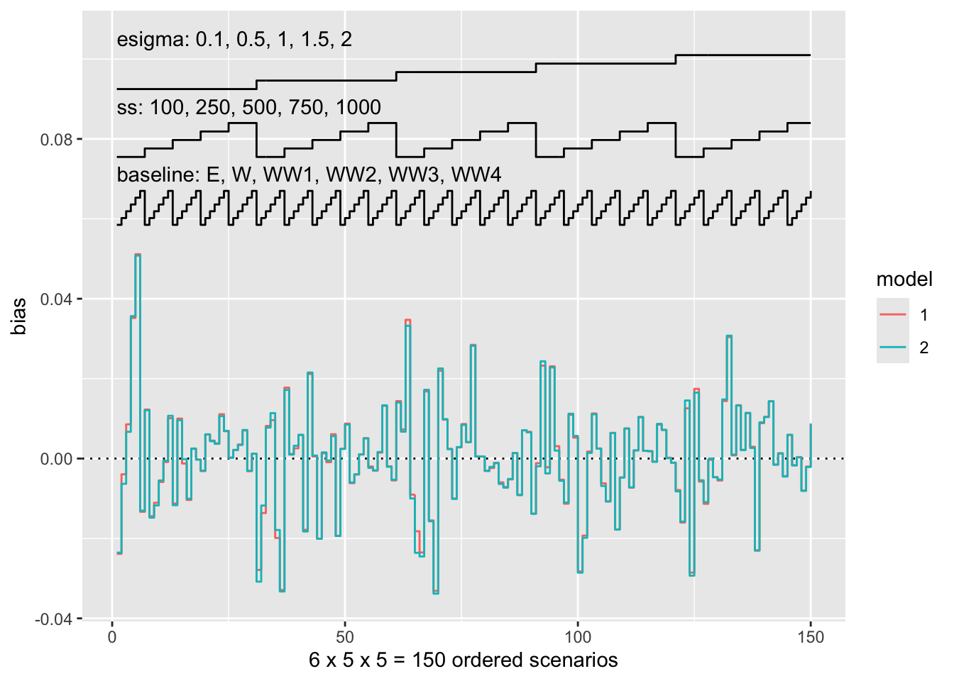

This has not changed since the previous release. If we however have an incomplete design, missing scenarios will now be empty:

nlp.subset <- subset(nlp, !(nlp$ss == 100 & nlp$esigma == 2))
s.nlp.subset <- simsum(
  data = nlp.subset,
  estvarname = "b",
  true = 0,
  se = "se",
  methodvar = "model",
  by = c("baseline", "ss", "esigma")
)
autoplot(s.nlp.subset, stats = "bias", type = "nlp")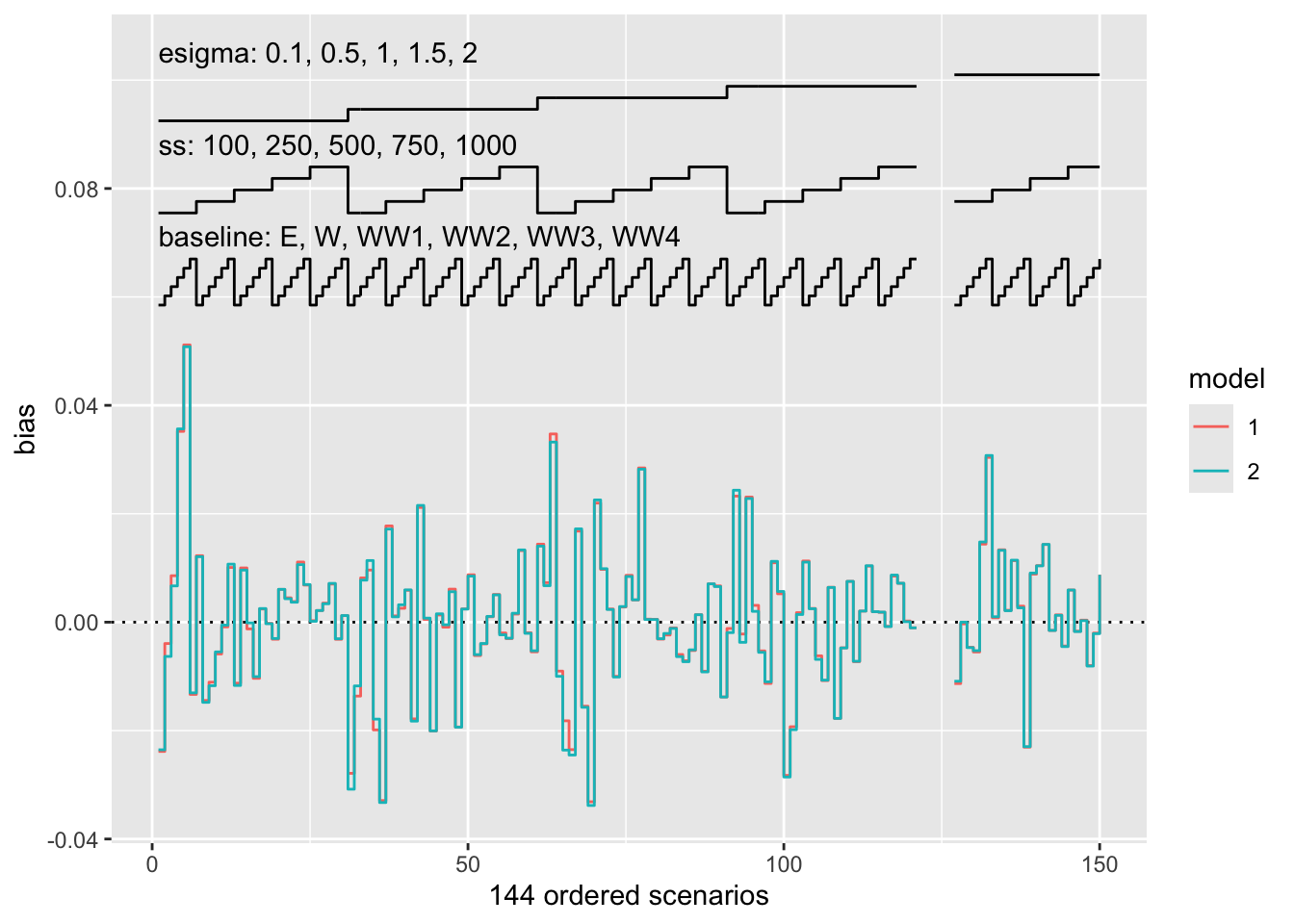

This should allow using nested loop plots in a wider variety of scenarios. Many thanks to Mike Sweeting for the suggestion.

Zipper plots

Lastly, it is now possible to further customise the appearance of zipper plots; specifically, the horizontal lines that are used to denote the estimated confidence intervals (based on Monte Carlo errors) of coverage probability under each scenario. The default behaviour hasn’t changed, with yellow bands:

data(relhaz, package = "rsimsum")
relhaz <- subset(relhaz, relhaz$baseline == "Weibull" & relhaz$model != "RP(2)")
s.zip <- simsum(
  data = relhaz,
  estvarname = "theta",
  se = "se",
  true = -0.50,
  methodvar = "model",
  by = "n",
  x = TRUE
)
autoplot(s.zip, type = "zip")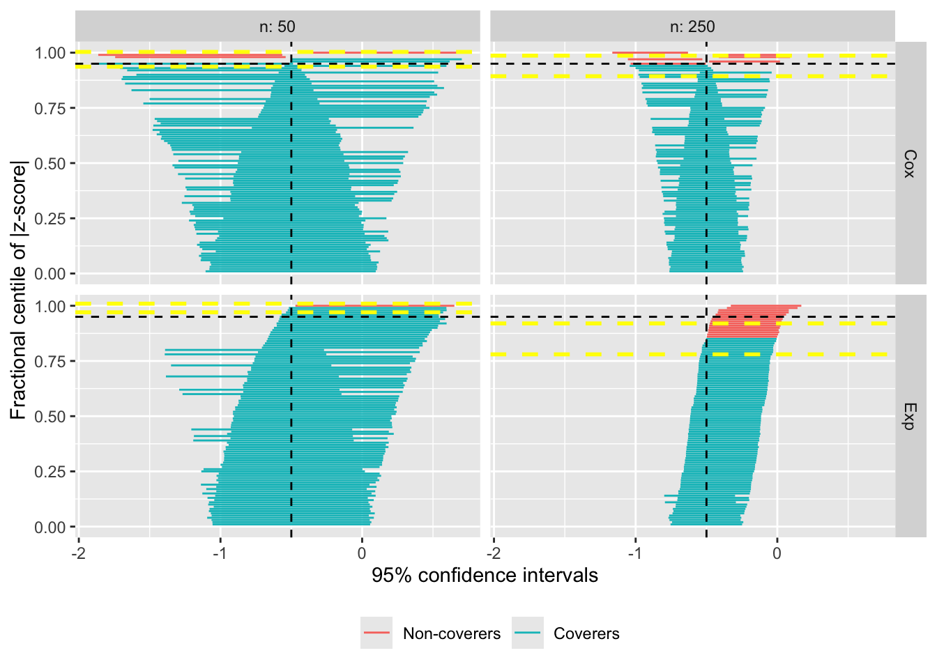

What is nice is that now you can use the zip_ci_colors argument of autoplot() to customise this. If you pass a single colour name (or hex value), that will be used throughout:

autoplot(s.zip, type = "zip", zip_ci_colours = "purple")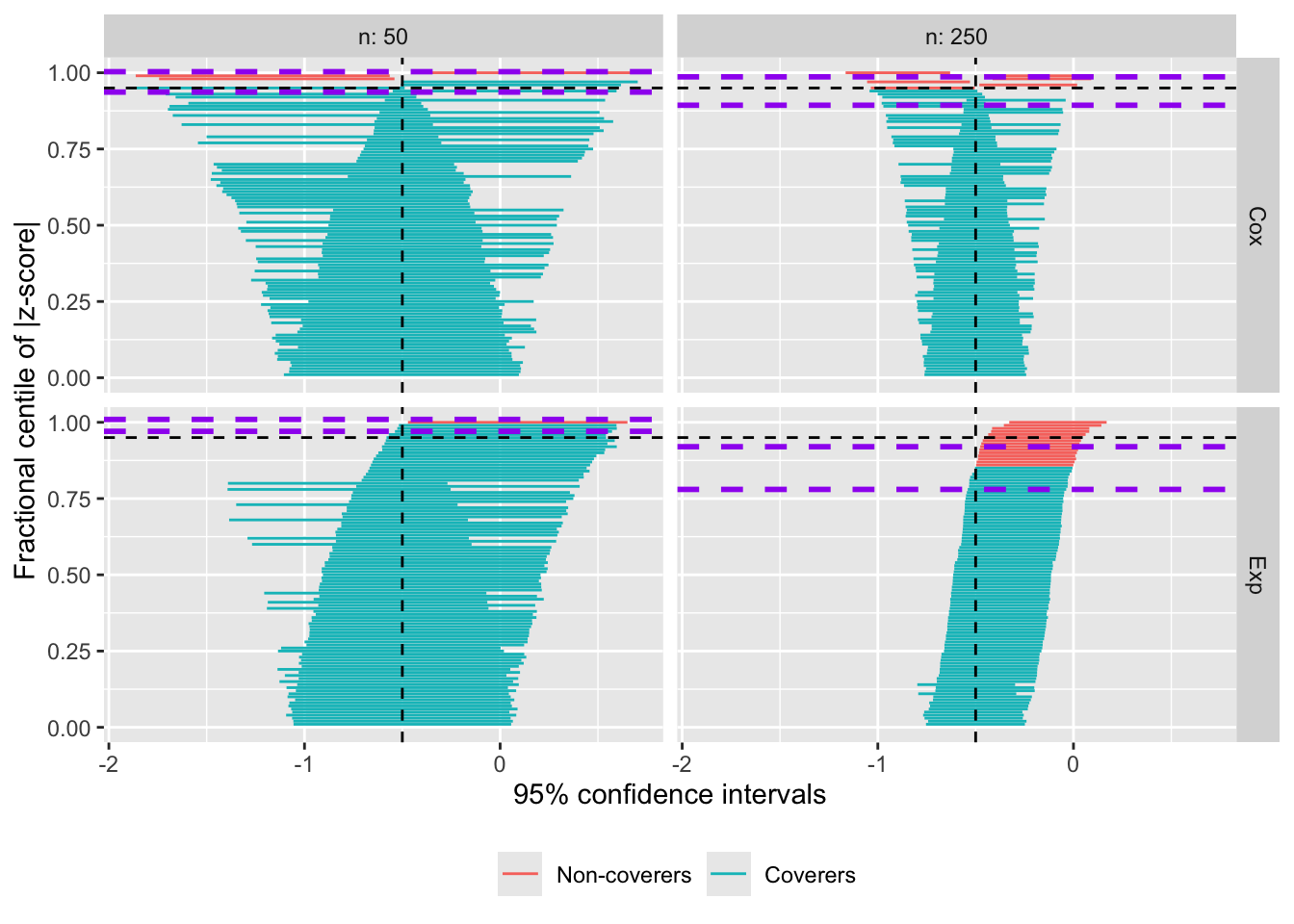

If you pass two values, those will be used for optimal and sub-optimal coverage, respectively:

autoplot(s.zip, type = "zip", zip_ci_colours = c("green", "red"))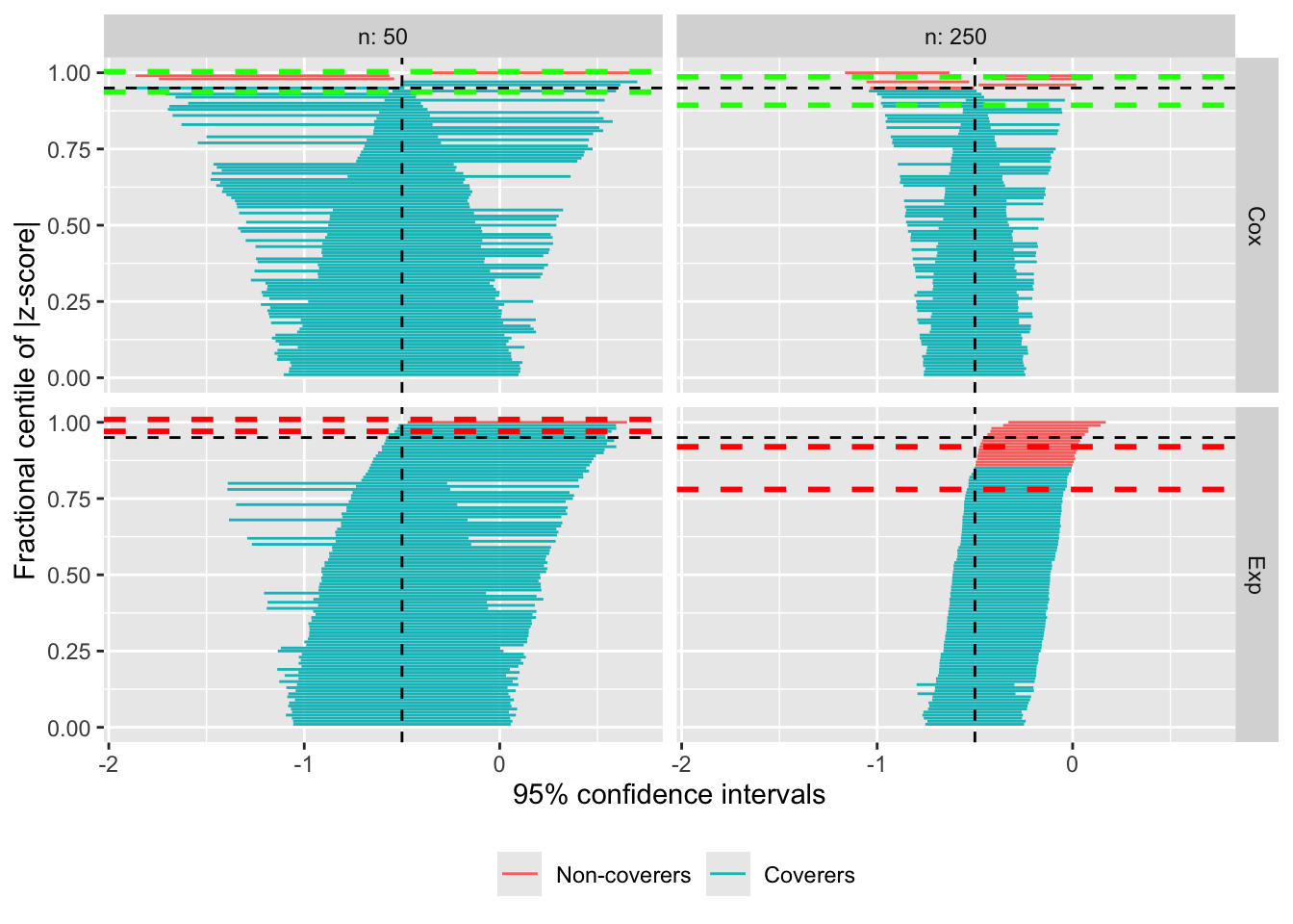

Finally, if you pass three values, those will be used for optimal coverage, under-coverage, and over-coverage, respectively:

autoplot(s.zip, type = "zip", zip_ci_colours = c("green", "blue", "red"))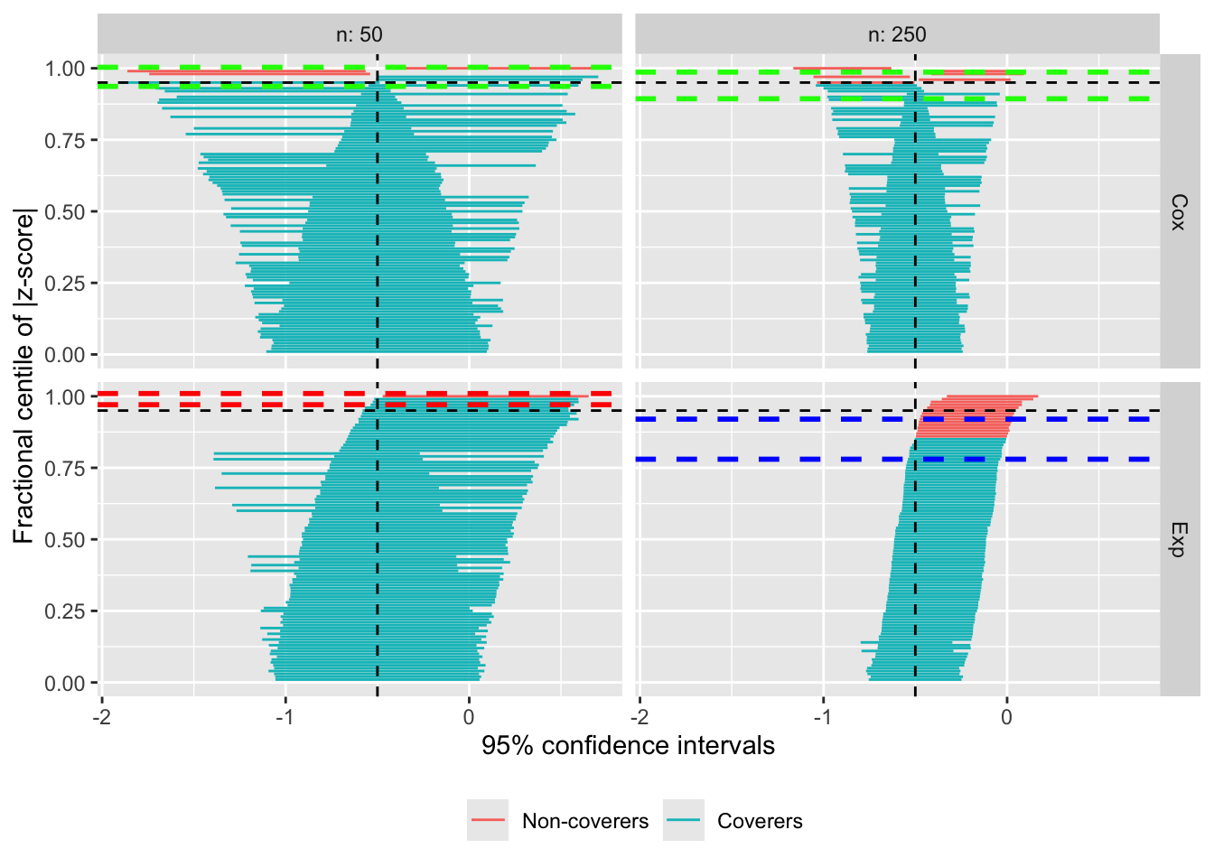

Of course, I would suggest picking better colours for a publication-worthy plot, but you get the gist. Many thanks to Lorenzo Guizzaro for the suggestion.