Today we will be talking about simulation studies and Monte Carlo errors. Yeah, I know, you heard it all before, but trust me… there will be something interesting in here, I swear!
Let’s start with the basics: Monte Carlo simulation is a stochastic procedure, thus for each run of a simulation study, we are likely to get slightly different results. And that’s fine! However, we want to be able to reproduce simulation results. Sure, we could set the seed of the random numbers generator, but what if we want the results to be similar regardless of what seed we set?
This concept is often referred to as statistical reproducibility: in other words, we want to minimise simulation error for results to be similar across replications.
This simulation error is often referred to as Monte Carlo error. And as you might already know, the {rsimsum} package can calculate Monte Carlo error for a variety of performance measures, such as bias.
However, what if you want to calculate Monte Carlo error for any potential performance measure out there? Well, today is your lucky day: as suggested by White, Royston, and Wood (2011) in the settings of multiple imputation, we can calculate the Monte Carlo error using a jackknife procedure to our simulation results. That is, the Monte Carlo error for any performance measure will be the standard error of the mean of the pseudo values for that statistic, computed by omitting one simulation repetition at a time.
Throughout this post, I will introduce all the above concepts, and I will show you how to use the jackknife to compute the Monte Carlo standard error for relative bias. We will also validate our calculations, which is always a good thing to do!
Jackknife resampling
The jackknife technique is, technically speaking, a cross-validation technique and thus it can be considered to be a form of resampling. Specifically, given a sample of size n, a jackknife estimator can be built by aggregating the parameter estimates from each subsample of size (n - 1), where the nth observation is omitted each time. Loosely speaking, this is not far from the concept of leave-one-out cross-validation.
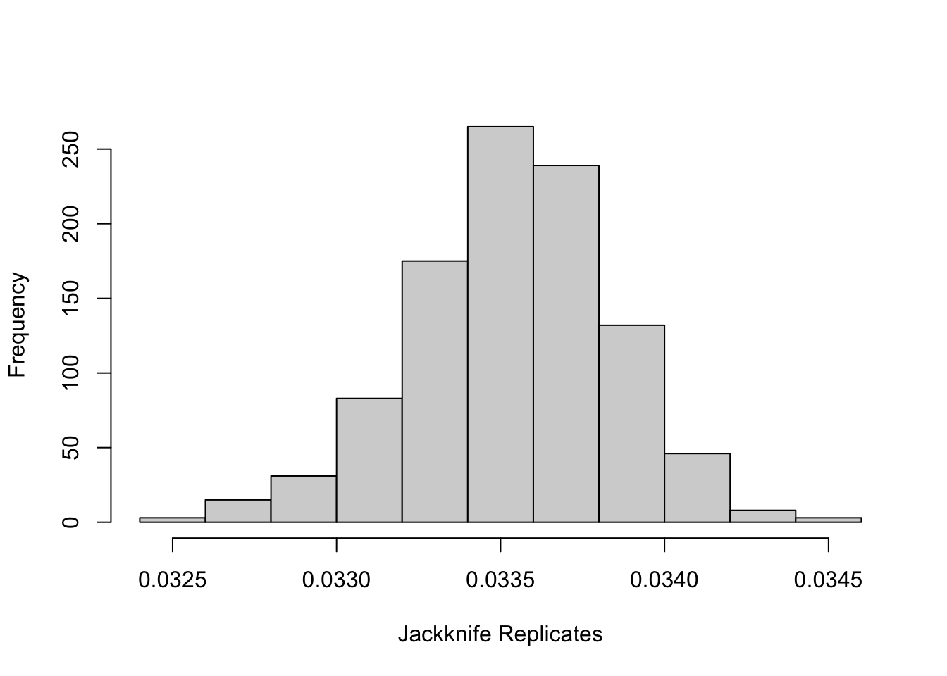
If we define a given statistics θ, for a sample of size n, we can calculate n jackknife replicates, denoted with θn, each computed by omitting the nth observation. Then, we can calculate the mean and the variance (and thus standard error) of such jackknife replicates, and there you go.
We now move on to relative bias. First, let’s define bias: according to Morris, White, and Crowther, that is defined (for a certain estimand θ) as: \[
E[\hat{\theta}] - \theta
\] and estimated by \[
\frac{1}{n} \sum_i \hat{\theta}_i - \theta,
\] assuming n repetitions.
This is routinely computed (and reported) for, anecdotally, most simulation studies in the literature. However, the magnitude of bias depends on the magnitude of θ; it is thus not necessarily easy to compare across studies with different data-generating mechanisms. That’s why it is sometimes interesting to compute relative bias, usually defined as \[
\frac{E[\hat{\theta}] - \theta}{\theta}
\] and estimated by \[
\frac{1}{n} \sum_i \frac{\hat{\theta}_i - \theta}{\theta}
\] The obvious downside is that relative bias, as defined here, cannot be calculated when the true θ = 0, but that’s beyond the scope of this blog post.
Let’s not illustrate how to use the jackknife to calculate the Monte Carlo standard error of relative bias. To do so, we will use a dataset that comes bundled with {rsimsum} for illustration purposes:
library(rsimsum)data("MIsim")str(MIsim)
tibble [3,000 × 4] (S3: tbl_df/tbl/data.frame)
 $ dataset: num [1:3000] 1 1 1 2 2 2 3 3 3 4 ...
 $ method : chr [1:3000] "CC" "MI_T" "MI_LOGT" "CC" ...
 $ b      : num [1:3000] 0.707 0.684 0.712 0.349 0.406 ...
 $ se     : num [1:3000] 0.147 0.126 0.141 0.16 0.141 ...
 - attr(*, "label")= chr "simsum example: data from a simulation study comparing 3 ways to handle missing"
MIsim <-subset(MIsim, MIsim$method =="CC")
Remember that, for this specific dataset, the true value of the estimand is θ = 0.5. We will also be using a single method (in this case, CC) for simplicity, but this can obviously be generalised. Bias can be easily computed using the simsum() function:
  stat        est        mcse       lower      upper
1 bias 0.01676616 0.004778676 0.007400129 0.02613219
Once again, this is exactly the same, which is good.
Actually…
It turns out, we don’t actually need the jackknife to obtain Monte Carlo standard errors (MCSE) for relative bias (RB). It can be shown (as usual, exercise left to the reader) that we can obtain a closed-form formula:
where RB hat is the estimated relative bias computed using the estimator above. Let’s compare this with the jackknife estimate. First, recall the estimated MCSE using the jackknife:
If you are still not convinced, let me show you something else. What is another method that one could use to estimate standard errors for any statistics you can pretty much think of? Well, but of course, it’s our best friend the bootstrap!
Let’s use non-parametric bootstrap to calculate the standard error of our relative bias estimator. For that, we use the {boot} package in R:
library(boot)set.seed(387456)rbfun <-function(data, i, .true) mean((data[i] - .true) / .true)bse <-boot(data = MIsim$b, rbfun, .true =0.5, R =50000)
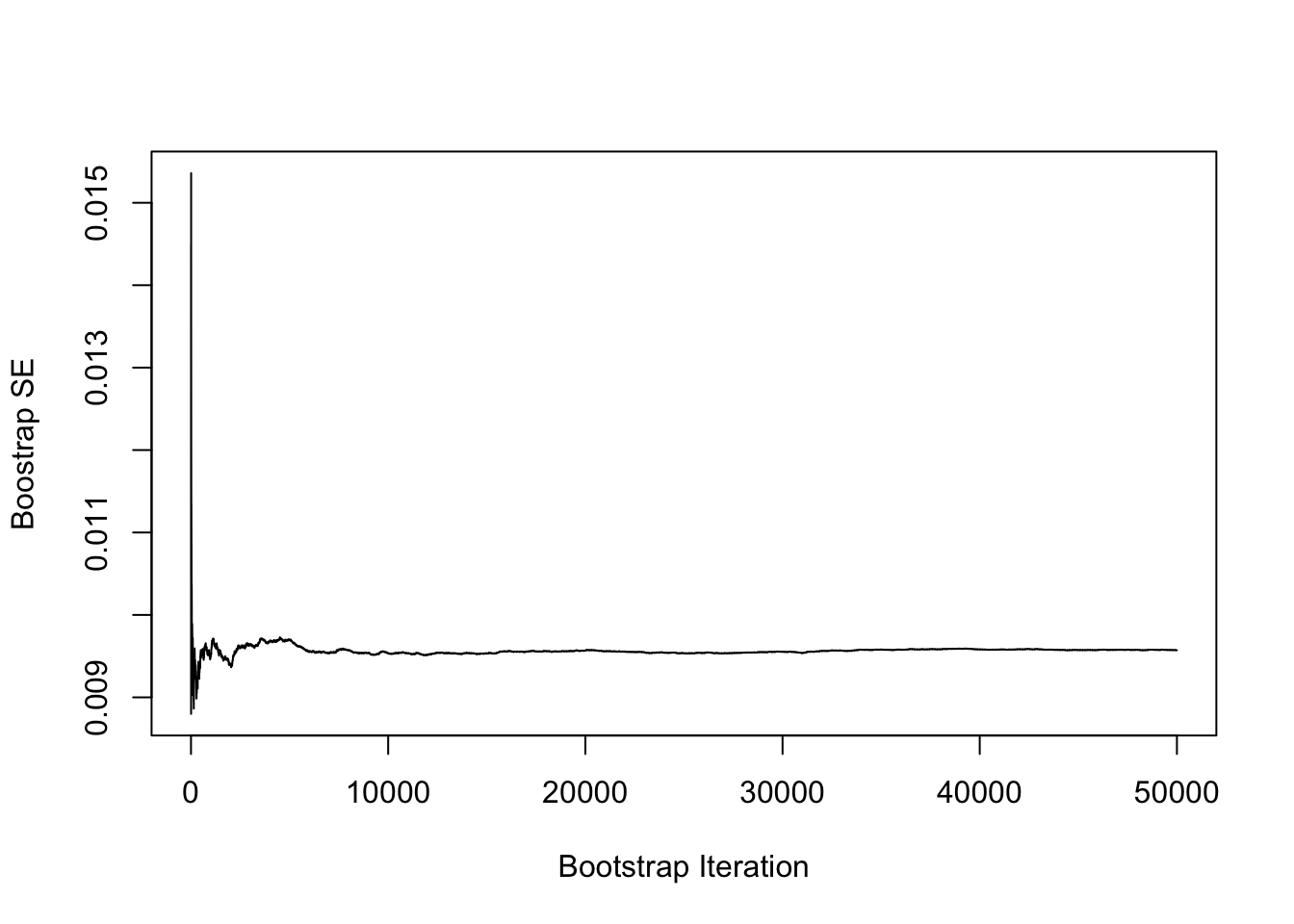
Note that rbfun() is a function we define to calculate relative bias, that we use R = 50000 bootstrap samples to ensure convergence of the procedure, and that we set a seed (for reproducibility). The results of the bootstrap are printed below:
Once again: pretty close, not exactly the same (as the bootstrap is still a stochastic procedure), but close enough that we can be confident that they converge to the same value.
Finally, let me reassure you that the bootstrap has converged (and, side note, you should remember to do that too when you use it):
…looks like the bootstrap converged, and that, probably, we did not need so many bootstrap samples after all. Luckily computations were so inexpensive that we could afford it (the whole thing took just a few seconds on my laptop), so that’s ultimately fine.
Wrap-up
And there you have it, examples of how to use the jackknife (and the bootstrap!) to estimate standard errors for a given metric of interest. Time to go wild and apply this to your settings!
In conclusion, I think these are very powerful tools that every statistician should be at least familiar with; there is plenty of literature on the topic, let me know if you’d like some references. Hope you learned something from this, I sure did by writing up all of this – and if you are still reading, here’s some breaking news:
Relative bias with Monte Carlo errors will be available in the next release of {rsimsum}! Coming soon to your nearest CRAN server…
Thanks for reading, and until next time, take care!