Numerical integration in generalised linear mixed models

Numerical integration in generalised linear mixed models (GLMMs): does the number of quadrature nodes matter?

Hi everyone!

I was in class a few weeks ago helping with a course on longitudinal data analysis, and towards the end of the course, we introduced generalised linear mixed models (GLMMs).

Loosely speaking, GLMMs generalise linear mixed models (LMMs) in the same way that generalised linear models (GLMs) extend the standard linear regression model: by allowing to model outcomes that follow distributions other than the gaussian, such as Poisson (e.g., for count data) or binomial (e.g., for binary outcomes – looking at you, logistic regression). Using proper notation, in GLMMs the response for the i^th subject at the j^th measurement occasion, \(Y_{ij}\), is assumed to follow any distribution from the exponential family such that \[ g[E(Y_{ij} | b_i)] = X_{ij} \beta + Z_{ij} b_i, \] where \(g(\cdot)\) is a known link function and \(b_i\) are the subject-specific random effects, assumed to follow a multivariate distribution with zero mean and variance-covariance matrix \(\Sigma\), \(b_i \sim N(0, \Sigma)\). Given that random effects are subject-specific, responses within each individual will be correlated.

Let’s go one step forward by defining the GLMM-equivalent of a logistic regression model, where the link function is a logistic function, and assuming a random intercept only (for simplicity): \[ \text{logit}[P(Y_{ij} = 1 | b_i)] = \beta X_{ij} + b_i, \ b_i \sim N(0, \nu^2) \] Here \(X_{ij}\) can represent any set of fixed effects covariates, such as a treatment assignment, time, or something like that, \(\beta\) a vector of regression coefficients, and \(b_i\) is univariately normal. Note that interpretation of the fixed effects is similar to that of regression coefficients from a logistic regression model, as they can be interpreted as log odds ratios. The main difference, however, is that this interpretation is conditional on random effects being set to zero – loosely speaking, this interpretation holds for an average subject (in terms of random effects). It is fundamentally important to keep this in mind when interpreting the results of LMMs and GLMMs!

To estimate a GLMM, we can use the maximum likelihood approach. The joint probability density function of \((Y_i, b_i)\) is given by \[ f(Y_i, b_i | X_i) = f(Y_i | b_i, X_i) f(b_i), \] where the random effect components are however latent (e.g., unobserved and unobservable). In order to calculate the individual contributions to the likelihood \(L_i\), we thus need to integrate out the density of the random effects: \[ L_i = \int_B f(Y_i | b_i, X_i) f(b_i) \ db_i \] …which unfortunately does not have a closed, analytical form for GLMMs.

Luckily, several methods have been proposed throughout the years to approximate the value of integrals that do not have a closed-form; this is generally referred to as numerical integration.

Now, this is where we go off a tangent; buckle up, boys.

Numerical integration

According to Wikipedia,

“[…] numerical integration comprises a broad family of algorithms for calculating the numerical value of a definite integral.”

As I mentioned above, the basic problem that numerical integration aims to solve is to approximate the value of a definite integral such as \[ \int_a^b f(x) \ dx \] to a given degree of accuracy.

The term numerical integration first appeared in 1915 (who knew?!) and, as you can imagine, a plethora of approaches have been proposed throughout the years to solve this problem.

Several approaches are based on deriving interpolating functions that are easy to integrate, such as polynomials of low degree (e.g., linear or quadratic). The simplest approach of this kind is the so-called rectangle rule (or midpoint rule), where the interpolating function is a constant function (i.e. 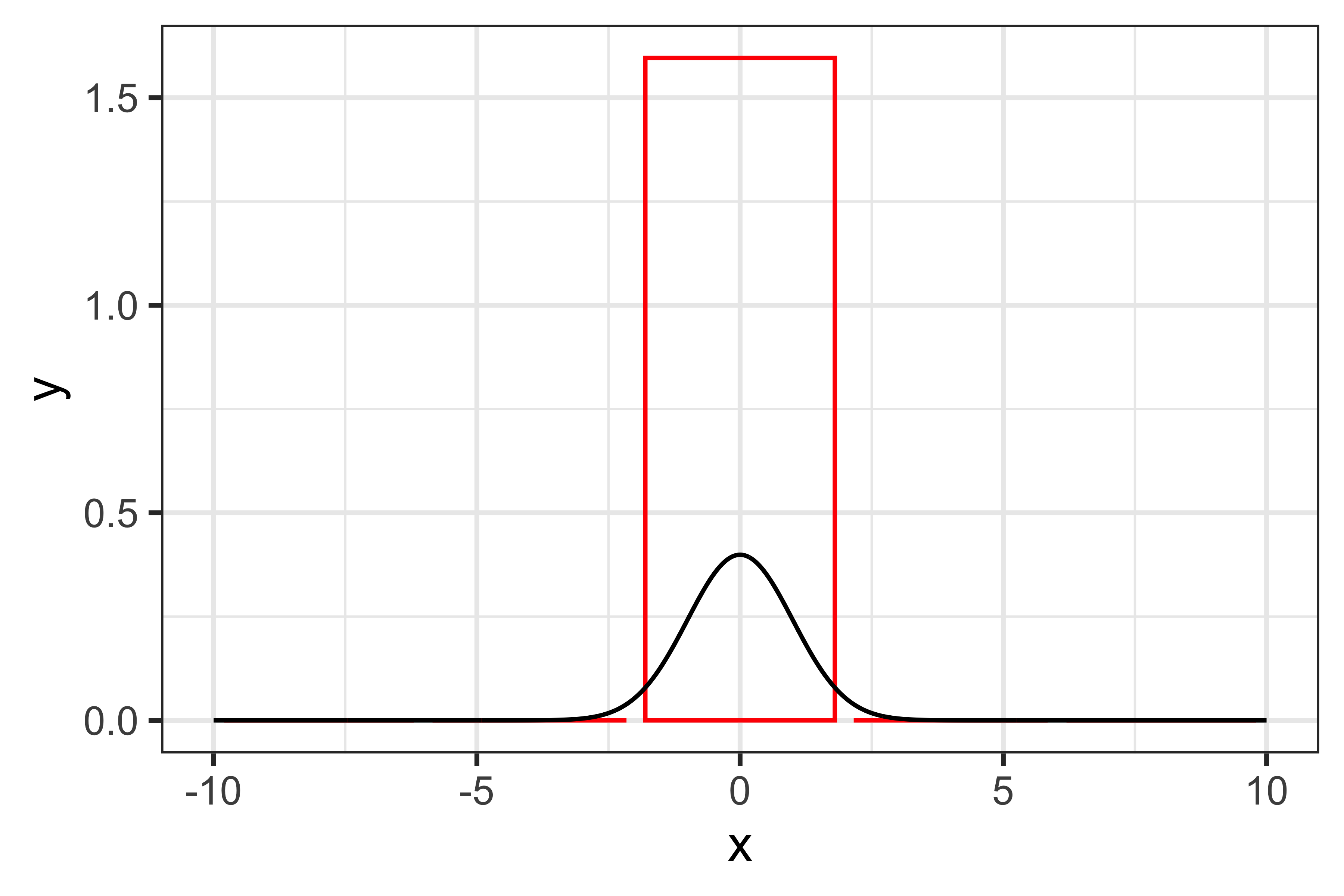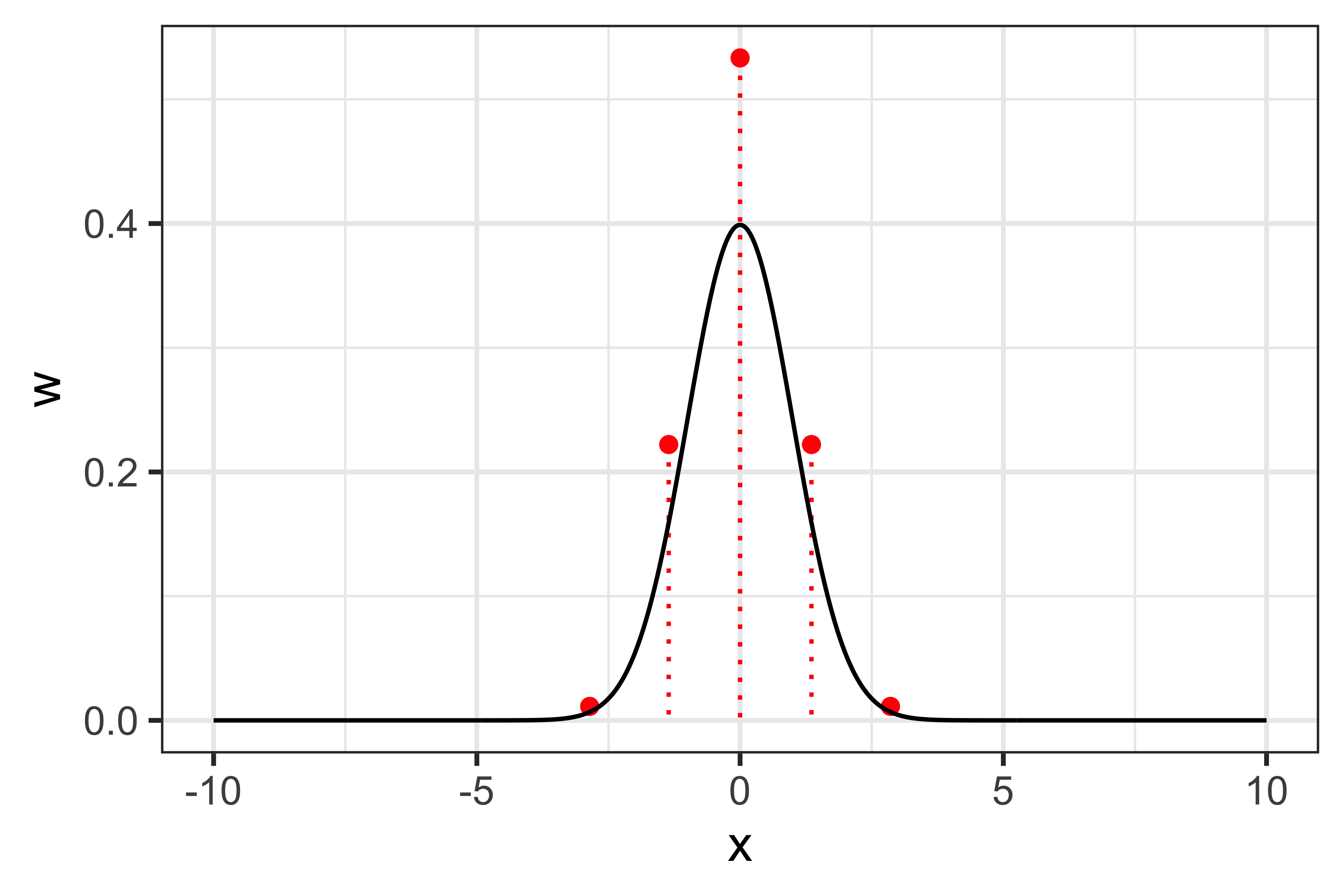a polynomial of degree zero) that passes through the midpoint: \[ \int_a^b f(x) \ dx \approx (b - a) f\left(\frac{a + b}{2}\right) \] Of course, the smart thing about this approach is that we can divide the integral into a large number of sub-intervals, thus increasing the accuracy of the approximation. Let’s illustrate this by assuming that we are trying to integrate a standard normal distribution (the dnorm() function in R), e.g. \(x \sim N(0, 1)\). With five sub-intervals, the approximation would look like:

And the approximated integral would be 1.59684 (the true value is one, given that we are integrating a distribution). With more sub-intervals, e.g. 15, the accuracy of this approximation improves:

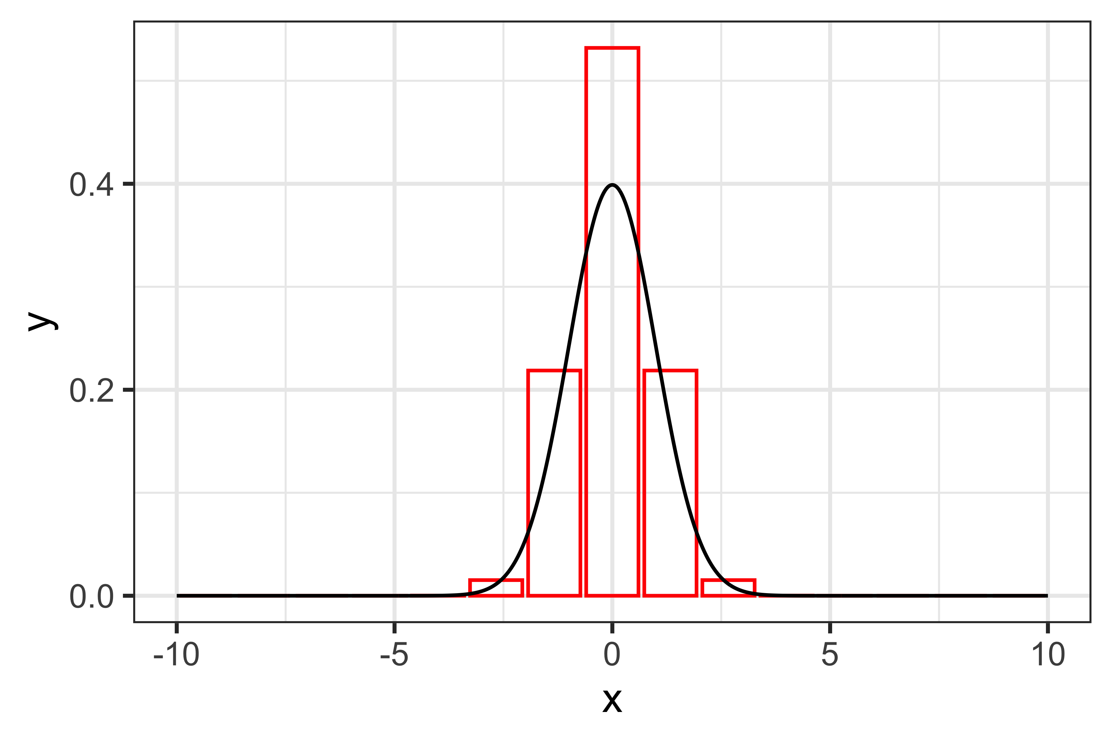
Now, the approximated integral is 1.00003, pretty much spot on. We can test how many sub-intervals are reguired to get a good approximation:

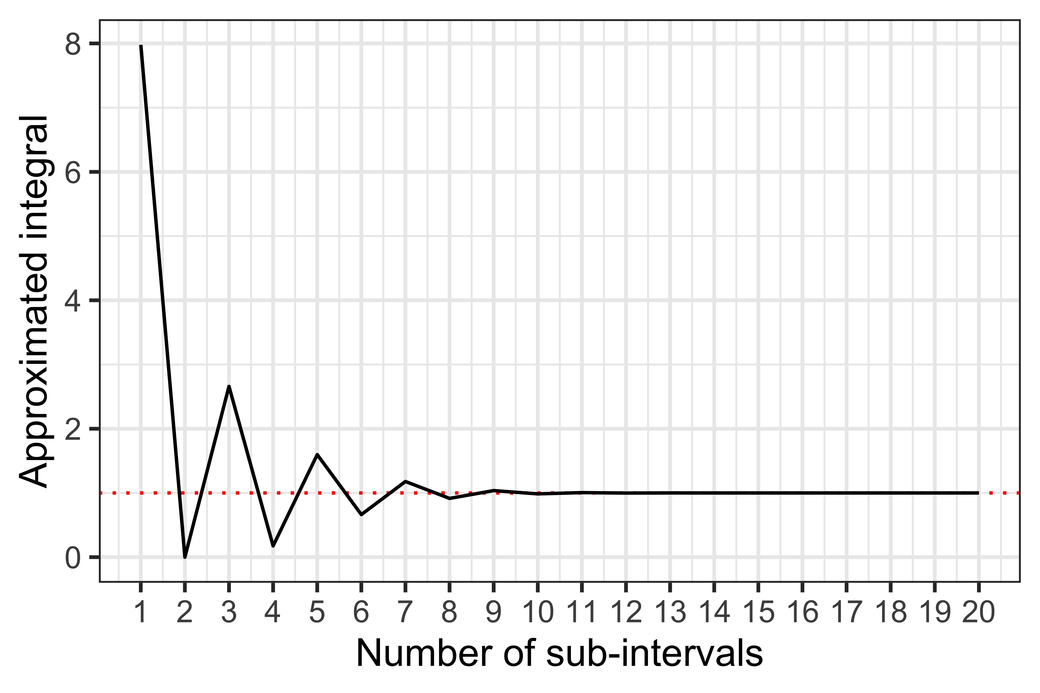
We can see that by using approximately 8-10 sub-intervals or more we can get a (very!) good approximation. Now, intuitively this works so well because we are trying to integrate a simple function; what if we had a more complex function, such as \[ f(x) = \frac{1}{(x + 1) \sqrt{x}}, \] that we want to integrate between zero and 20?

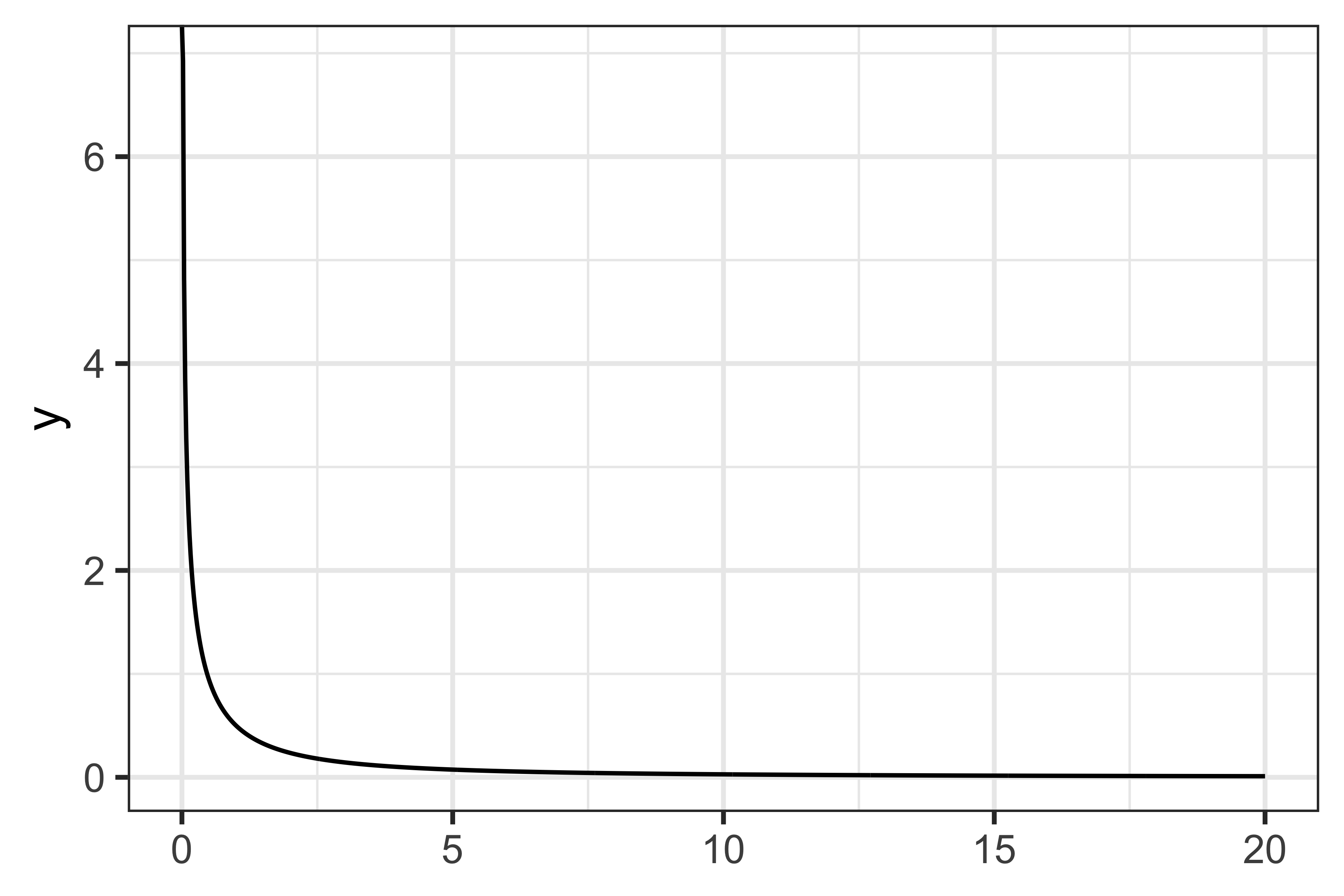
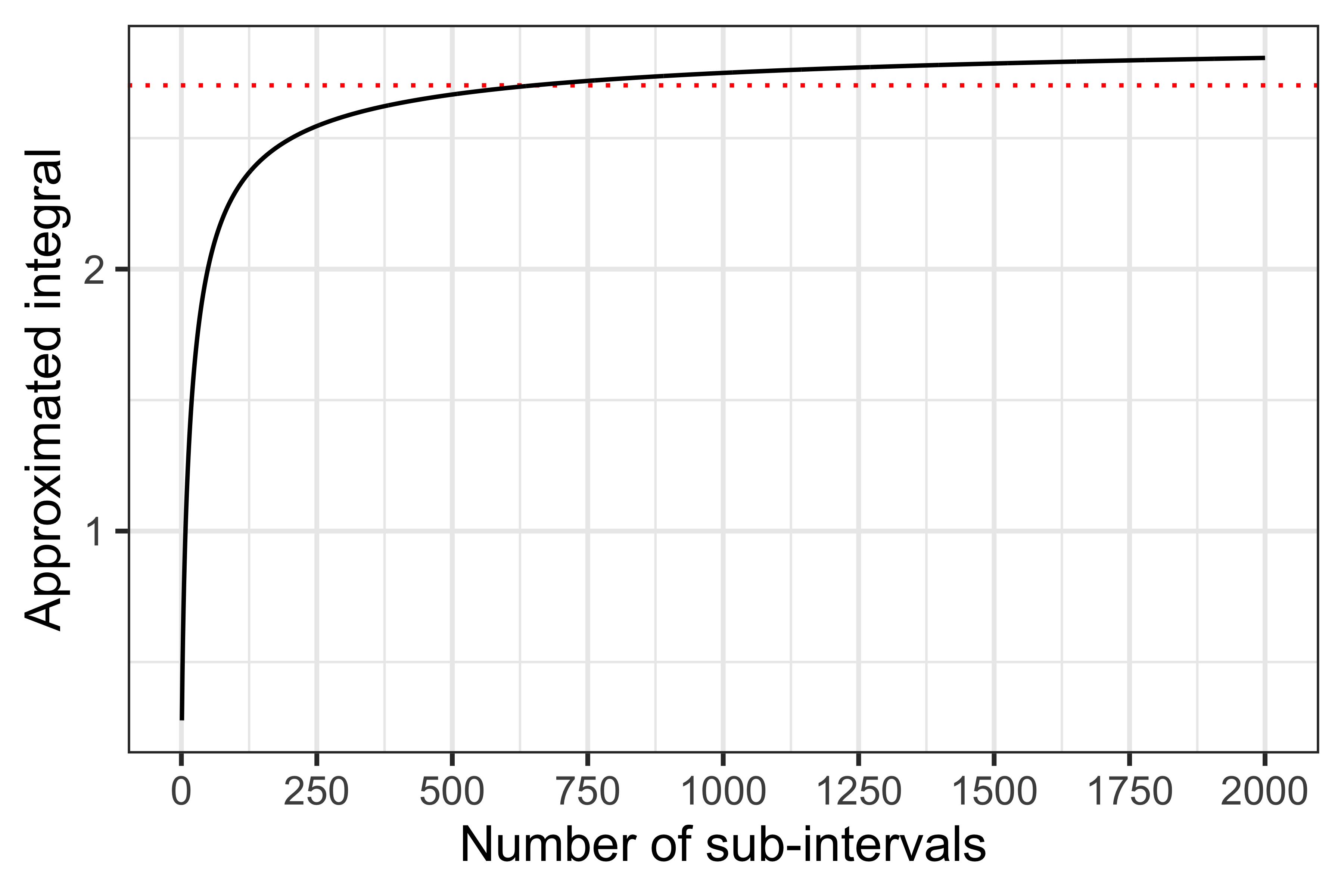
As you can see from the plot above, the performance here is much worse than before.

The simple rectangle rule can now be improved by using more complex interpolating functions (e.g., using a polynomial of degree one, leading to a trapezoidal rule, or a polynomial of degree two, leading to a Simpson’s rule). We will however jump a million steps ahead (…sorry! The Wikipedia article on numerical integration includes a bunch more details if you want to read more about this), and talk about more elaborate numerical integration methods that are actually used when estimating the likelihood function of a GLMM.

Specifically, two approaches are routinely used, the first of which is Laplace approximation. The Laplace approximation uses a second-order Taylor series expansion, based on re-writing the intractable integrand from the likelihood contributions, which allows deriving closed-form expressions for the approximation. This is generally the fastest approach, and it can be shown that the approximation is asymptotically exact for an increasing number of observations per random effect. See, e.g., here for more details on the Laplace approximation in the settings of GLMMs.

Nevertheless, in practical applications, the accuracy of the Laplace approximation may still be of concern. Thus, a second approach for numerical integration is often used to obtain more accurate approximations (while however being more computationally demanding): Gaussian quadrature.

A quadrature rule is an approximation of a definite integral of a function that is stated as a weighted sum of function values at specified points within the domain of integration. For instance, when integrating a function over the domain \([-1, 1]\), such rule (using \(n\) points) is defined as: \[ \int_{-1}^{1} f(x) \ dx \approx \sum_{i = 1}^{n} w_i f(x_i) \] This rule is exact for polynomials of degree \(2n - 1\) or less. For our specific problem, the domain of integration is \((-\infty, +\infty)\) (the domain of the normal distribution of the random effects); this leads to a so-called Gauss-Hermite quadrature rule, which given the normal distribution that we are trying to approximate, has optimal properties. Specifically, Gauss-Hermite integration with a function kernel of \(e^{-x^2}\) for a normal distribution with mean \(\mu\) and variance \(\sigma^2\), leads to the following rule: \[ \int_{-\infty}^{+\infty} f(x) \ dx \approx \sum_{i = 1} ^ n \frac{w_i}{\sqrt{\pi}} \phi(\sqrt{2} \sigma z_i + \mu), \] with \(\phi(\cdot)\) the density of a standard normal distribution (such as dnorm() in R).

Let’s get back to the example that we used above, integrating a standard normal distribution, to visualise Gauss-Hermite quadrature. This can be visualised, for 5-points quadrature, as:

For 11-points quadrature:

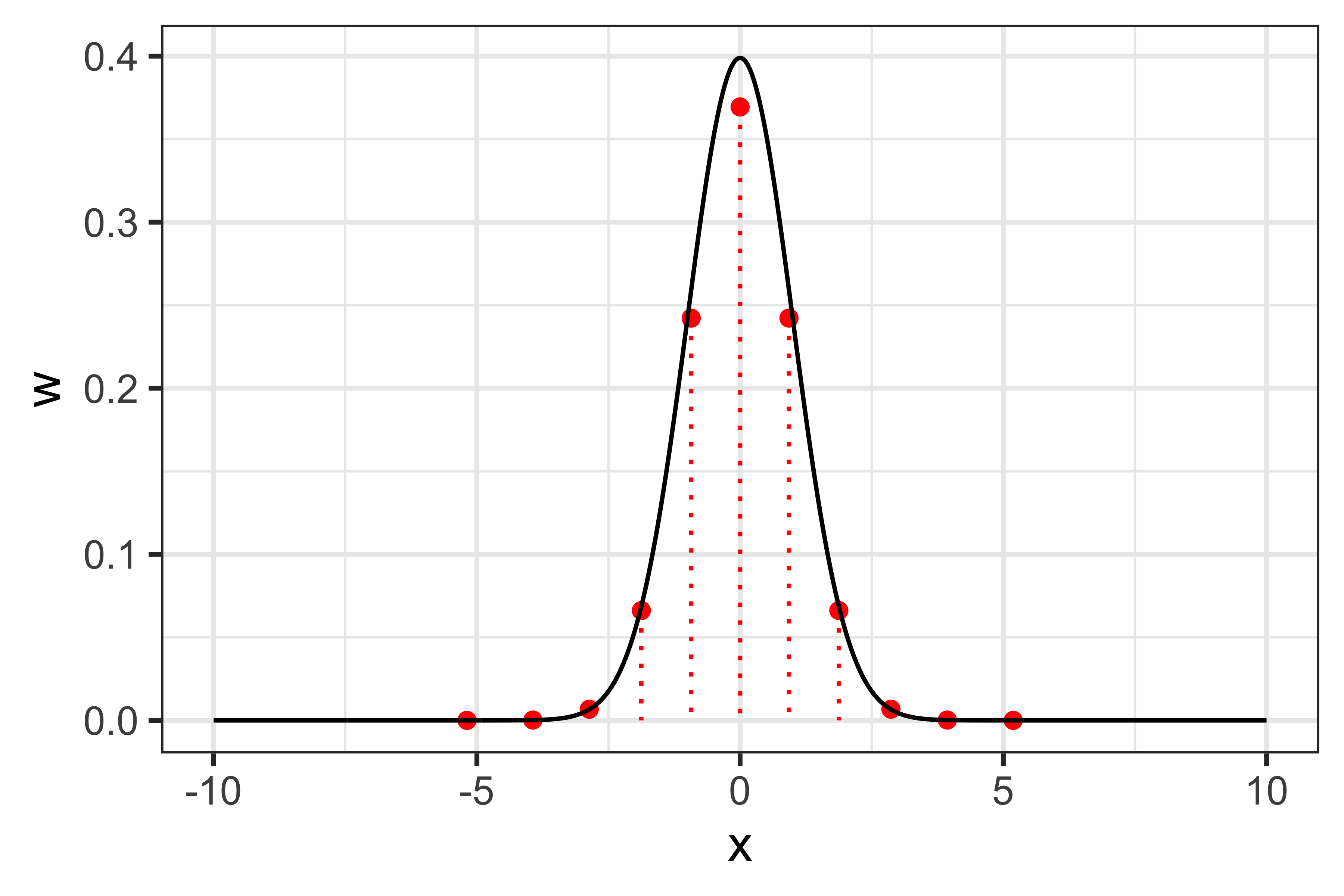
Testing convergence of this procedure:

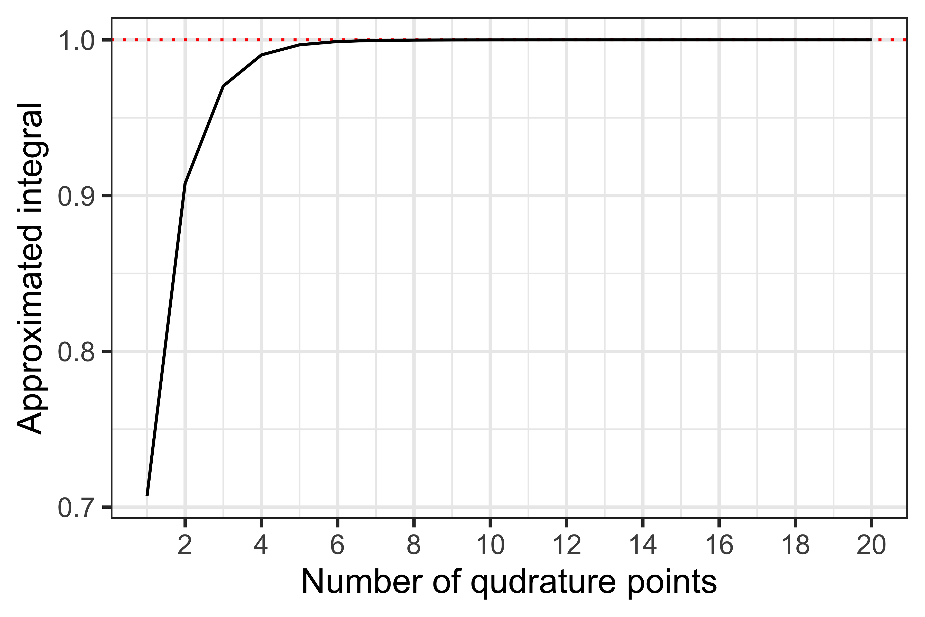
As before, already with 7 quadrature points we get a good approximation of the density. Anecdotally, a larger number of quadrature points might be required to get a good approximation in practice, which would require more function evaluations and therefore a larger computational burden. Furthermore, this problem becomes exponentially more complex in higher dimensions, e.g., with more than one random effect: a univariate quadrature rule with 5 points requires 5 function evaluations, while a bivariate one with the same number of points requires 5²=25 evaluations every single time the intractable integral is evaluated. Interestingly, Pinheiro and Bates showed that it is possible to adapt the integration procedure to be more computationally efficient in higher dimensions, by centring and scaling the quadrature procedure using conditional moments of the random effects distribution.

Now, we arrived at the end of this detour in the world of numerical integration; there are many more details that I skipped here, but the references linked above should provide a good starting point for the interested reader. Let’s get back to business.

Numerical integration in GLMMs

Remember that the individual contributions to the likelihood \(L_i\) for a GLMM are intractable, thus requiring numerical integration: \[ L_i = \int_B f(Y_i | b_i, X_i) f(b_i) \ db_i \]

By now you can probably appreciate that accuracy of this approximation is key, but in practical terms, what does this mean? In other words, what happens if we fail to accurately approximate that integral?

Yes, my friends, it is finally time to get to the meat of this post, a mere 2,000 words later!

Simulation? Simulation!

We can try to answer that question using statistical simulation. If you know me, you might have noticed that I think that simulations are a fantastic tool for learning about complex statistical concepts. What better than this to further prove the point, then?

Let’s start by describing the protocol of this simulation study. We use the ADEMP framework to structure the protocol (and if you’re not on the ADEMP bandwagon, jump on, there’s still some space left).

Aim

The aim of this simulation study is to test the accuracy of different numerical integration methods in terms of estimation of fixed and random effects in GLMMs.

Data-generating mechanism

We use a single data generating mechanism for simplicity. We simulate binary outcomes for the i^th subject, j^th occasion from the following data-generating model:

\[\text{logit}(Y_{ij} = 1) = (\beta_0 + b_{0i}) + \beta_1 \text{Treatment}_i + \beta_2 \text{Time}_{ij} + \beta_3 \text{Treatment}_i \times \text{Time}_{ij}\]

Note that:

1. We include a binary treatment which is assigned a random at baseline by drawing from a Bernoulli random variable with a success probability of 0.5;

2. Time between each measurement, in years, for each subject, is simulated by drawing from a Uniform(0, 1) random variable;

3. I allow for a maximum of 100 measurements per subject, and truncate follow-up after 10 years;

4. \(b_{0i}\) is a random intercept, simulated by drawing a subject-specific value from a normal distribution with mean zero and standard deviation \(\sigma_{b_0}\) = 4;

5. The regression parameters are assigned the values -2, -1, 0.5, and -0.1 for \(\beta_0\), \(\beta_1\), \(\beta_2\), and \(\beta_3\), respectively.

Finally, every simulated dataset includes 500 subjects.

Estimands

The estimands of interest are the regression parameters \(B = \{\beta_0, \beta_1, \beta_2, \beta_3\}\) and the standard deviation of the random intercept \(\sigma_{b_0}\).

Methods

We fit the true, data-generating GLMM as implemented in the glmer() function from the {lme4} package in R, where we vary, however, the numerical integration method. In glmer(), this is defined by the nAGQ argument. We use the following methods for numerical integration:

1. nAGQ = 0, corresponding to a faster but less exact form of parameter estimation for GLMMs by optimizing the random effects and the fixed-effects coefficients in the penalised iteratively reweighted least-squares step;

2. nAGQ = 1, corresponding to the Laplace approximation. This is the default for glmer();

3. nAGQ = k, with k number of points used for the adaptive Gauss-Hermite quadrature method. I test values of k from 2 to 10, and then from 15 to 50 at steps of 5, for a total of 17 possible values of k. Remember that, as the glmer() documentation points out, larger values of k produce greater accuracy in the evaluation of the log-likelihood at the expense of speed.

In total, 19 models are fit to each simulated dataset and compared with this simulation study.

Performance measure

The main performance measure of interest is bias in the estimands of interest, to test the accuracy of the different numerical integration methods.

Number of repetitions

An important issue to keep in mind when running simulation studies is that of Monte Carlo error. Loosely speaking, there is a certain amount of randomness in the simulation and therefore uncertainty in the estimation of the performance measures of interest, thus we have to make sure that we can estimate them accurately (e.g., with low Monte Carlo error). This can be done iteratively, e.g., by running repetitions until the Monte Carlo error drops below a certain threshold (see here for more details).

For simplicity, we take a different approach here. What we do is the following:

1. Running 20 repetitions of this simulation study;

2. Using these 20 repetitions to estimate empirical standard errors and average model-based standard errors, for each estimand, and taking the largest value (denoted with \(\xi\));

3. Using the value that was just estimated to estimate how many repetitions would be needed to constrain Monte Carlo error to be less than 0.01, using the formula n_sim = \(\xi / (0.01^2)\);

4. Rounding up the value of n_sim to the nearest 100, to be conservative.

n_sim was finally estimated to be 1700, in this case, given \(\xi \approx 0.1607\).

Results

At last, here are the results of this simulation study.

First, we assess whether all Monte Carlo errors for bias are below the threshold of 0.01. The plot below shows that the number of repetitions of this simulation study was enough to constrain Monte Carlo error within what we deemed acceptable.

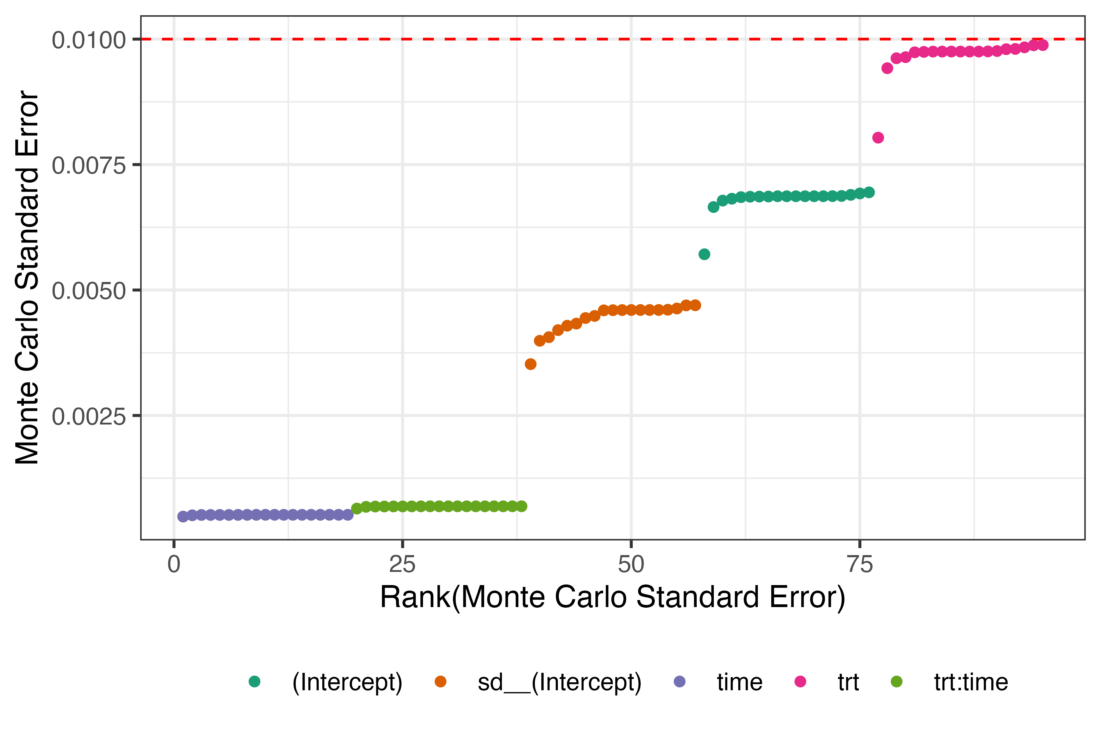
Note that (Intercept) corresponds to \(\beta_0\), trt corresponds to \(\beta_1\), time corresponds to \(\beta_2\), and trt:time corresponds to \(\beta_3\). Unsurprisingly, sd__(Intercept) represents the standard deviation of the random intercept, \(\sigma_{b_0}\).

Second, we study bias for the fixed effects (e.g., the regression coefficients of the GLMM). The following plot depicts bias with 95% confidence intervals (based on Monte Carlo standard errors) for all fixed effects and across all integration methods:

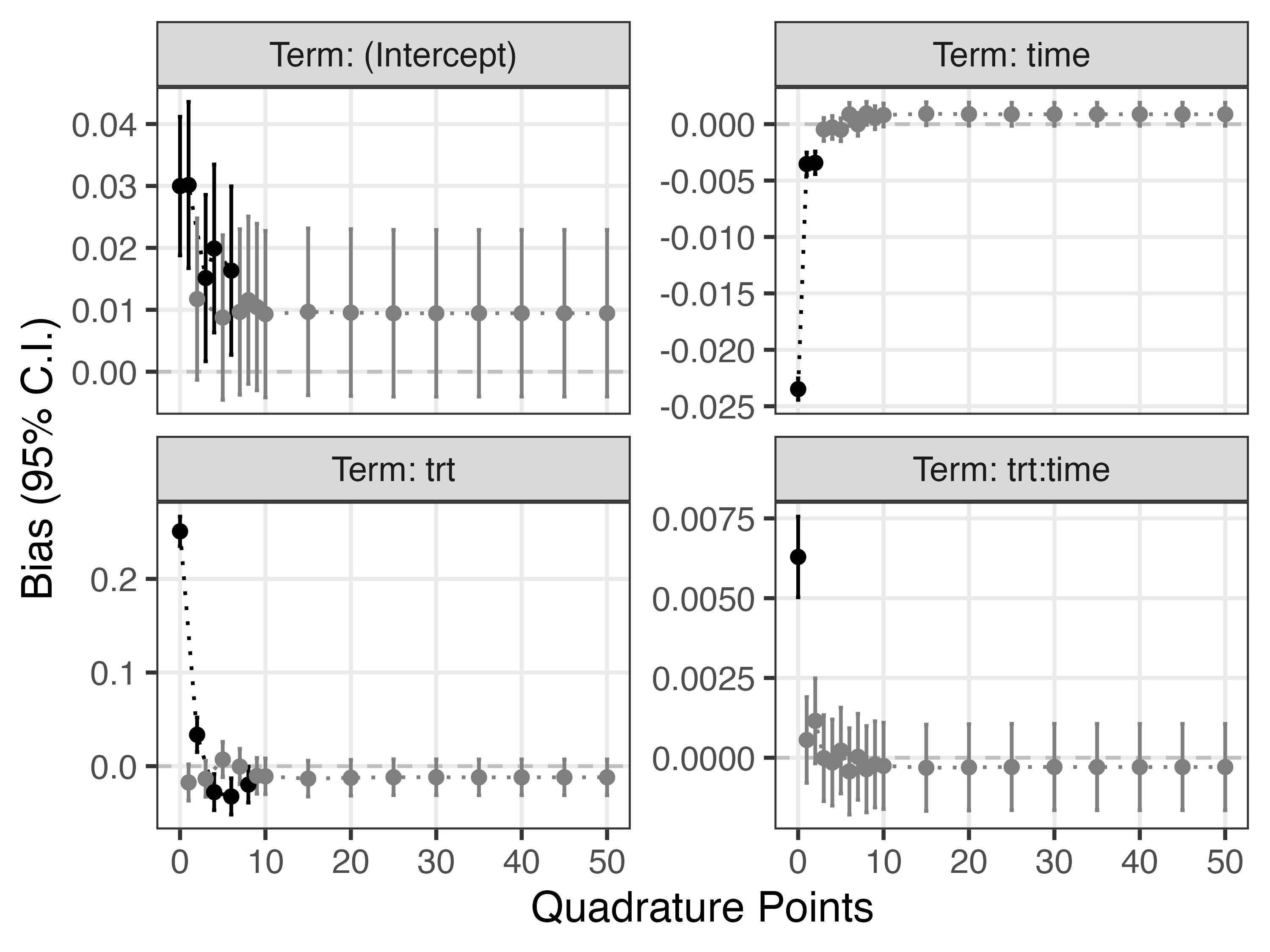
This shows that the fast-but-approximate method yields biased results, and that so does the Laplace approximation (in these settings, and except for the treatment by time interaction term). Overall, this shows that a larger number of points for the adaptive quadrature (e.g., 10) is required to obtain unbiased results for all regression coefficients.

Finally, the next plot shows bias for the standard deviation of the random intercept:

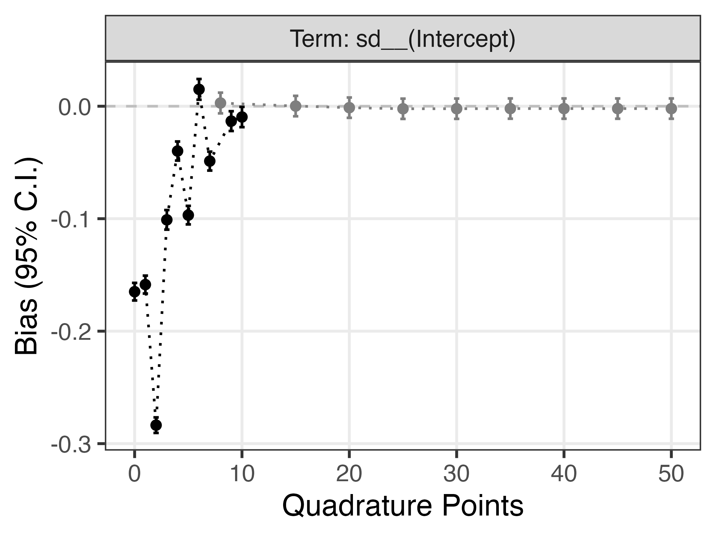
Again, we can see that a larger number of quadrature points is required to get a good approximation with no bias.

Another thing that is interesting to study here is estimation time. As mentioned many times before, the larger the number of quadrature points the greater the accuracy, at the cost of additional computational complexity. But how much overhead do we have in these settings?

I’m glad you asked: the following plot depicts the distribution of estimation times for each GLMMs under each integration approach:

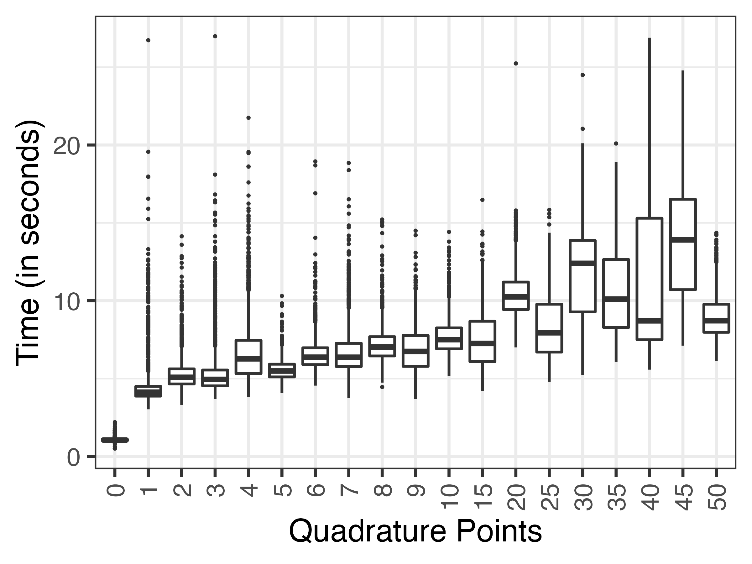
The first thing to note is that the fast-but-approximate method is actually really fast! Second, and as expected, with more quadrature points the median estimation time was also larger. No surprises so far. Overall, though, glmer() seemed to be really fast in the settings, with estimation times rarely exceeding 25 seconds.

An actual example

Before we wrap up, let’s compare the different methods in practice by analysing a real dataset. For this, we use data from the 1989 Bangladesh fertility survey, which can be obtained directly from Stata:

library(haven)
library(dplyr)

bangladesh <- read_dta("http://www.stata-press.com/data/r17/bangladesh.dta")
glimpse(bangladesh)

Rows: 1,934
Columns: 8
$ district <dbl> 1, 1, 1, 1, 1, 1, 1, 1, 1, 1, 1, 1, 1, 1, 1, 1, 1, 1, 1, 1, 1…
$ c_use    <dbl+lbl> 0, 0, 0, 0, 0, 0, 0, 0, 0, 0, 1, 0, 0, 0, 0, 1, 0, 1, 1, …
$ urban    <dbl+lbl> 1, 1, 1, 1, 1, 1, 1, 1, 1, 1, 1, 1, 1, 1, 1, 1, 1, 1, 1, …
$ age      <dbl> 18.440001, -5.559990, 1.440001, 8.440001, -13.559900, -11.559…
$ child1   <dbl> 0, 0, 0, 0, 0, 0, 0, 0, 1, 0, 0, 0, 1, 0, 0, 0, 0, 0, 1, 0, 0…
$ child2   <dbl> 0, 0, 1, 0, 0, 0, 0, 0, 0, 0, 0, 0, 0, 0, 0, 0, 0, 0, 0, 1, 0…
$ child3   <dbl> 1, 0, 0, 1, 0, 0, 1, 1, 0, 1, 0, 0, 0, 1, 1, 1, 0, 1, 0, 0, 0…
$ children <dbl+lbl> 3, 0, 2, 3, 0, 0, 3, 3, 1, 3, 0, 0, 1, 3, 3, 3, 0, 3, 1, …

We will fit a GLMM model for a binary outcome trying to study contraceptive use by urban residence, age and number of children; we also include a random intercept by district.

For illustration purposes, we fit three models:

1. GLMM estimated with the fast-but-approximate (nAGQ = 0) approach;

2. GLMM estimated with the Laplace approximation (nAGQ = 1);

3. GLMM estimated with adaptive Gauss-Hermite quadrature using 50 points (nAGQ = 50).

The models can be fit with the following code:

library(lme4)

f.0 <- glmer(c_use ~ urban + age + child1 + child2 + child3 + (1 | district), family = binomial(), data = bangladesh, nAGQ = 0)
f.1 <- glmer(c_use ~ urban + age + child1 + child2 + child3 + (1 | district), family = binomial(), data = bangladesh, nAGQ = 1)
f.50 <- glmer(c_use ~ urban + age + child1 + child2 + child3 + (1 | district), family = binomial(), data = bangladesh, nAGQ = 50)

…and we use the {broom.mixed} package to tidy, summarise, and compare the results from the three models:

library(broom.mixed)
library(ggplot2)

bind_rows(
  tidy(f.0, conf.int = TRUE) %>% mutate(nAGQ = "f.0"),
  tidy(f.1, conf.int = TRUE) %>% mutate(nAGQ = "f.1"),
  tidy(f.50, conf.int = TRUE) %>% mutate(nAGQ = "f.50")
) %>%
  ggplot(aes(x = nAGQ, y = estimate)) +
  geom_errorbar(aes(ymin = conf.low, ymax = conf.high), width = 1 / 3) +
  geom_point() +
  scale_y_continuous(n.breaks = 5) +
  theme_bw(base_size = 12) +
  facet_wrap(~term, scales = "free_y") +
  labs(x = "Method (nAGQ)", y = "Point Estimate (95% C.I.)")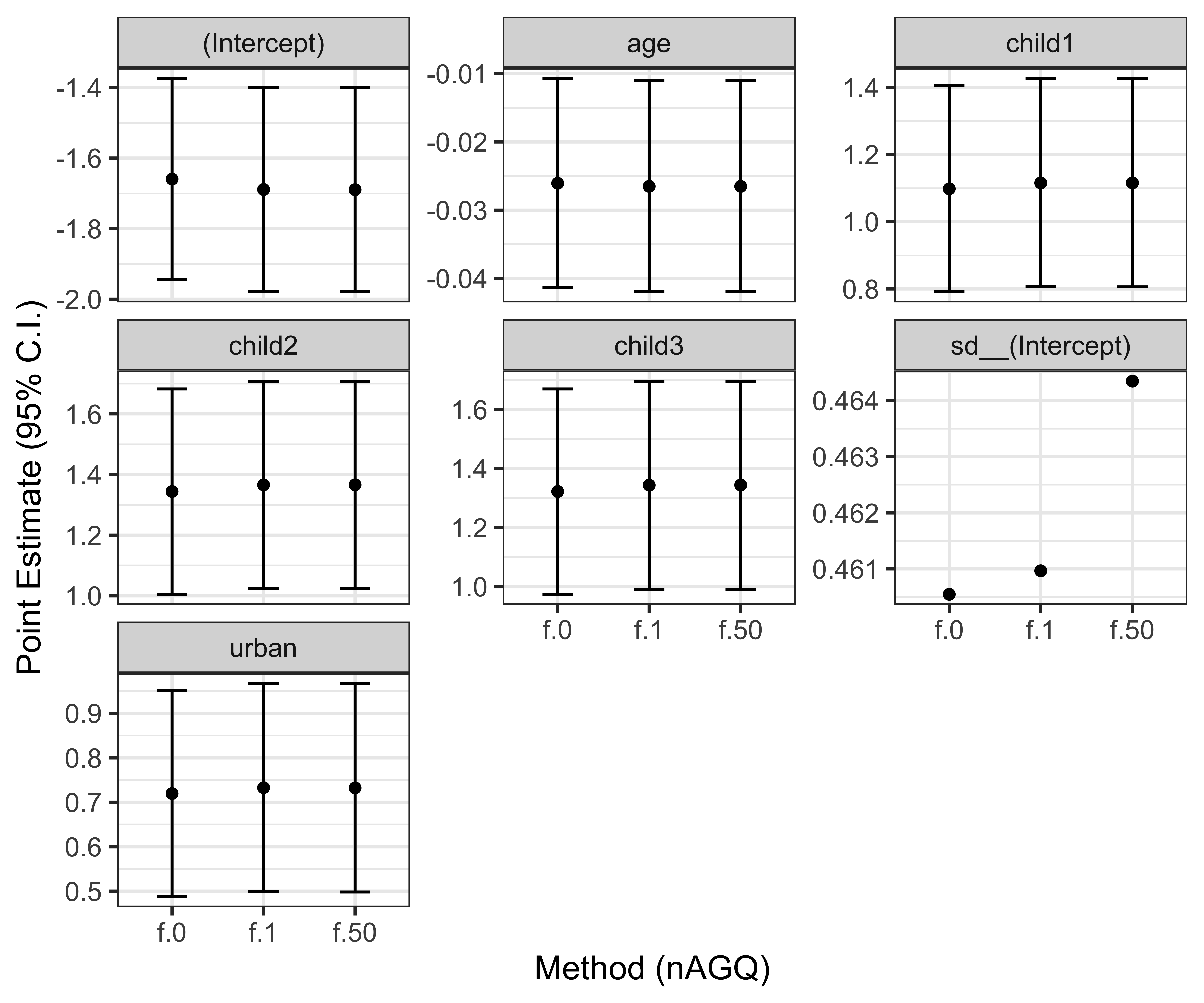

Model coefficients from the three integration approaches are very similar in this case, thus we can be confident that the results of this analysis are likely not affected by that. Let’s thus print the summary of the model using adaptive quadrature:

summary(f.50)

Generalized linear mixed model fit by maximum likelihood (Adaptive
  Gauss-Hermite Quadrature, nAGQ = 50) [glmerMod]
 Family: binomial  ( logit )
Formula: c_use ~ urban + age + child1 + child2 + child3 + (1 | district)
   Data: bangladesh

     AIC      BIC   logLik deviance df.resid 
  2427.7   2466.6  -1206.8   2413.7     1927 

Scaled residuals: 
    Min      1Q  Median      3Q     Max 
-1.8140 -0.7662 -0.5087  0.9973  2.7239 

Random effects:
 Groups   Name        Variance Std.Dev.
 district (Intercept) 0.2156   0.4643  
Number of obs: 1934, groups:  district, 60

Fixed effects:
             Estimate Std. Error z value Pr(>|z|)    
(Intercept) -1.689295   0.147759 -11.433  < 2e-16 ***
urban        0.732285   0.119486   6.129 8.86e-10 ***
age         -0.026498   0.007892  -3.358 0.000786 ***
child1       1.116005   0.158092   7.059 1.67e-12 ***
child2       1.365893   0.174669   7.820 5.29e-15 ***
child3       1.344030   0.179655   7.481 7.37e-14 ***
---
Signif. codes:  0 '***' 0.001 '**' 0.01 '*' 0.05 '.' 0.1 ' ' 1

Correlation of Fixed Effects:
       (Intr) urban  age    child1 child2
urban  -0.288                            
age     0.449 -0.044                     
child1 -0.588  0.054 -0.210              
child2 -0.634  0.090 -0.382  0.489       
child3 -0.751  0.093 -0.675  0.538  0.623

Furthermore, we can interpret exponentiated fixed effect coefficients as odds ratios:

exp(fixef(f.50))

(Intercept)       urban         age      child1      child2      child3 
  0.1846497   2.0798277   0.9738498   3.0526345   3.9192232   3.8344665 

This shows that contraceptive use is higher in urban versus rural areas, with double the odds, that older women have lower odds of using contraceptives, and that the odds of using contraceptives are much higher in women with one or more children (odds ratios between 3 and 4 for women with 1, 2, or 3 children versus women with no children) – all else being equal. Nonetheless, remember that these results are conditional on a random intercept of zero, e.g., loosely speaking, for an average district.

Finally, there is also significant heterogeneity in contraceptive use between districts, with a variance for the random intercept of 0.2156. The distribution of the (log-) baseline odds of contraceptive use across districts can be visualised as:

ggplot(data = coef(f.50)$district, aes(x = `(Intercept)`)) +
  geom_density() +
  theme_bw(base_size = 12) +
  labs(x = "Baseline log-odds of contraceptive use", y = "Density")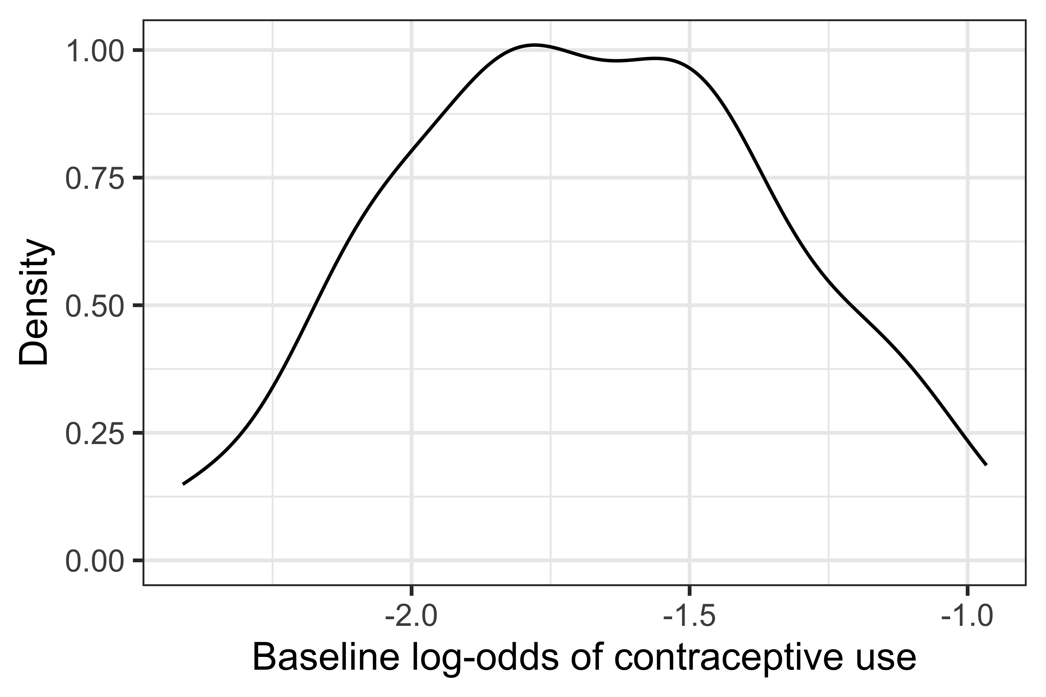

Closing thoughts

In conclusion, we saw how easy it is to get biased fixed effect estimates in GLMMs if we use a numerical integration method that is not accurate enough. Of course, this is just a single scenario and not a comprehensive study of estimation methods for GLMMs, but it should nonetheless show the importance of considering the estimation procedure when using (somewhat) more advanced statistical methods. This is, unfortunately, often overlooked in practice. My friendly suggestion would be to fit multiple models with different integration techniques, and if no significant differences are observed, then great: you got yourself some results that are robust to the numerical integration method being used.

This wraps up the longest blog post I’ve ever written (at ~3,500 words): if you made it this far, thanks for reading, and I hope you found this educational. And as always, please do get in touch if I got something wrong here.

Finally, R code for the simulation study, if you want to replicate the analysis or adapt it to other settings, is of course freely available on a GitHub repository here.

Cheers!