Assessing convergence of a simulation study

rsimsum

simulation

convergence

Describing an approach for assessing convergence of a Monte Carlo simulation study.

Published

December 31, 2021

Hey everyone,

The blog is back! And just in time to wrap up 2021.

Let’s get straight to business, shall we? Today we’re going to talk about ways of assessing whether your simulation study has converged. This is something that’s been on my mind for a while, and I finally got some focused time to write about it.

To do so, let’s first define what we mean with converged:

We define a simulation study as converged if:

Estimation of our key performance measures is stable, and

Monte Carlo error is small enough.

We are going to use the MIsim dataset, which you should be familiar with by now if you’ve been here before, and which comes bundled with the {rsimsum} package:

library(rsimsum)
data("MIsim", package = "rsimsum")
head(MIsim)

# A tibble: 6 × 4
  dataset method      b    se
    <dbl> <chr>   <dbl> <dbl>
1       1 CC      0.707 0.147
2       1 MI_T    0.684 0.126
3       1 MI_LOGT 0.712 0.141
4       2 CC      0.349 0.160
5       2 MI_T    0.406 0.141
6       2 MI_LOGT 0.429 0.136

To find out more about this data, type ?MIsim in your R console after loading the {rsimsum} package.

Interestingly, this dataset already includes a column named dataset indexing each repetition of the simulation study. If that was not the case, we should create such a column at this stage.

Let’s also load the {tidyverse} package for data wrangling and visualisation with {ggplot2}:

library(tidyverse)

The first step consists of computing performance measures cumulatively, e.g. for the first i repetitions (where i goes from 10 to the total number of repetitions that we run for our study, in this case, 1000). We use 10 here as the starting point as we assume that we should run at least 10 repetitions to get any useful result.

This can be easily done using our good ol’ friend the simsum function and map_ from the {purrr} package; specifically, we use map_dfr() to get a dataset obtained by stacking rows instead of a list object. Notice also that we only focus on bias as the performance measure of interest here; this could be done, in principle, for any other performance measure.

full_results <- map_dfr(
  .x = 10:1000,
  .f = function(i) {
    s <- simsum(
      data = filter(MIsim, dataset <= i),
      estvarname = "b",
      se = "se",
      true = 0.5,
      methodvar = "method",
      ref = "CC"
    )
    s <- summary(s)
    results <- rsimsum:::tidy.summary.simsum(s)
    results <- filter(results, stat == "bias") %>%
      mutate(i = i)
    return(results)
  }
)
head(full_results)

  stat         est       mcse  method       lower      upper  i
1 bias 0.006621292 0.04267397      CC -0.07701815 0.09026074 10
2 bias 0.016931728 0.03830584 MI_LOGT -0.05814635 0.09200980 10
3 bias 0.008187965 0.03047714    MI_T -0.05154612 0.06792205 10
4 bias 0.009806267 0.03873124      CC -0.06610556 0.08571810 11
5 bias 0.021526182 0.03495223 MI_LOGT -0.04697892 0.09003129 11
6 bias 0.016194059 0.02870663    MI_T -0.04006990 0.07245802 11

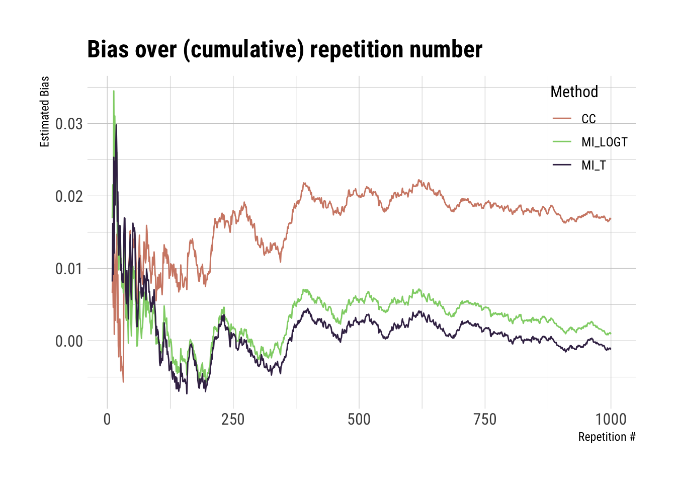
We can use these results to plot estimated bias (and corresponding Monte Carlo standard errors) over repetition numbers:

library(hrbrthemes) # Provide some nicer themes and colour scales

ggplot(full_results, aes(x = i, y = est, color = method)) +
  geom_line() +
  scale_color_ipsum() +
  theme_ipsum_rc(base_size = 12) +
  theme(legend.position = c(1, 1), legend.justification = c(1, 1)) +
  labs(x = "Repetition #", y = "Estimated Bias", color = "Method", title = "Bias over (cumulative) repetition number")

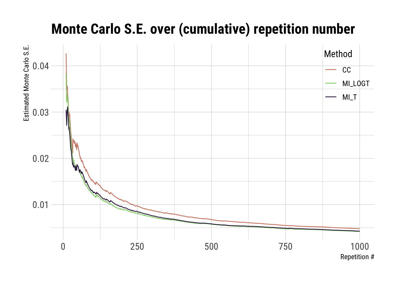
ggplot(full_results, aes(x = i, y = mcse, color = method)) +
  geom_line() +
  scale_color_ipsum() +
  theme_ipsum_rc(base_size = 12) +
  theme(legend.position = c(1, 1), legend.justification = c(1, 1)) +
  labs(x = "Repetition #", y = "Estimated Monte Carlo S.E.", color = "Method", title = "Monte Carlo S.E. over (cumulative) repetition number")

What shall we be looking for in these plots?

Basically, if (and when) the curves flatten. Remember flatten the curve? That applies here as well.

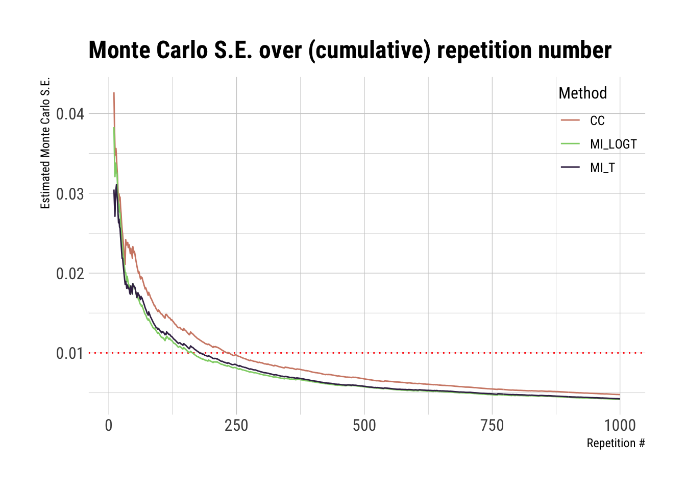
For Monte Carlo standard errors, we want to also check when they reach a threshold of uncertainty (e.g. 0.01) that we are willing to accept. We can also add this threshold to the plot to help our intuition:

ggplot(full_results, aes(x = i, y = mcse, color = method)) +
  geom_hline(yintercept = 0.01, color = "red", linetype = "dotted") +
  geom_line() +
  scale_color_ipsum() +
  theme_ipsum_rc(base_size = 12) +
  theme(legend.position = c(1, 1), legend.justification = c(1, 1)) +
  labs(x = "Repetition #", y = "Estimated Monte Carlo S.E.", color = "Method", title = "Monte Carlo S.E. over (cumulative) repetition number")

The plots above seem to be stable enough after ~500 repetitions, while Monte Carlo errors cross our threshold after ~250 repetitions. If I had to interpret this, I would be satisfied with the convergence of the study.

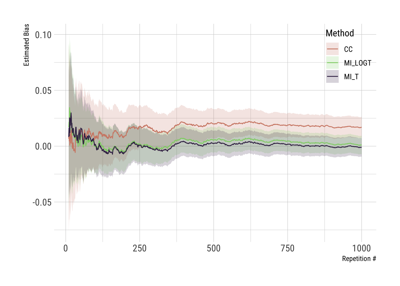
The dataset with results (full_results) includes confidence intervals for estimated bias, at each (cumulative) repetition number, based on Monte Carlo standard errors. We can, therefore, further enhance the first plot introduced above:

ggplot(full_results, aes(x = i, y = est)) +
  geom_ribbon(aes(ymin = lower, ymax = upper, fill = method), alpha = 1 / 5) +
  geom_line(aes(color = method)) +
  scale_fill_ipsum() +
  scale_color_ipsum() +
  theme_ipsum_rc(base_size = 12) +
  theme(legend.position = c(1, 1), legend.justification = c(1, 1)) +
  labs(x = "Repetition #", y = "Estimated Bias", color = "Method", fill = "Method")

Adding confidence intervals surely enhances our perception of stability.

Now, we could stop here and call it a day, but where’s the fun in that? Let’s take it to the next level.

I think that an even better way of assessing convergence is to check whether the incremental value of an additional repetition affects the results of the study (or not). When running additional repetitions stop adding value (e.g. changing the results), then we can (safely?) assume we have converged to stable results.

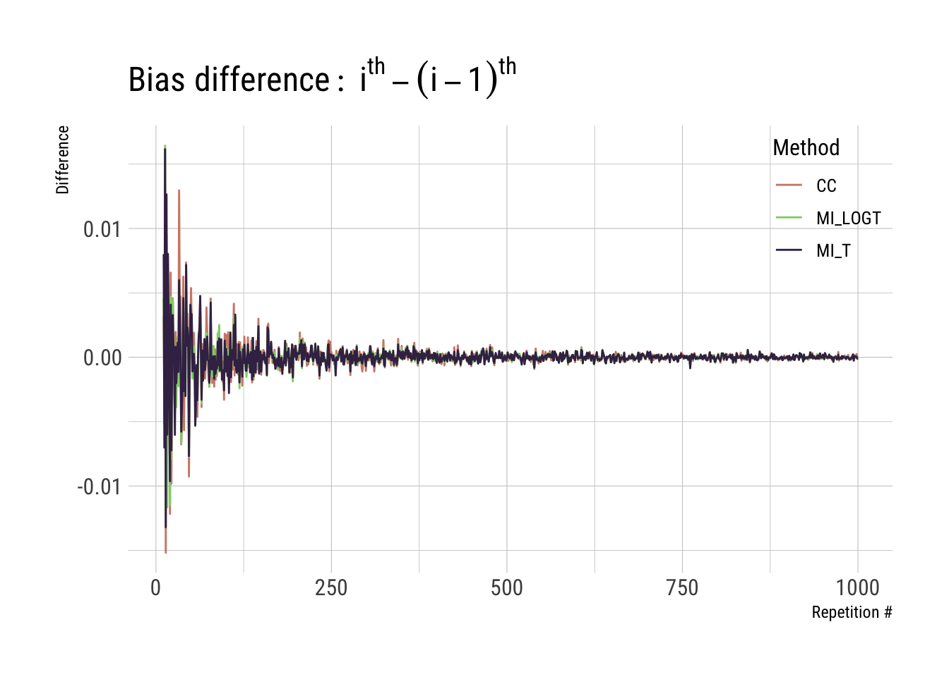
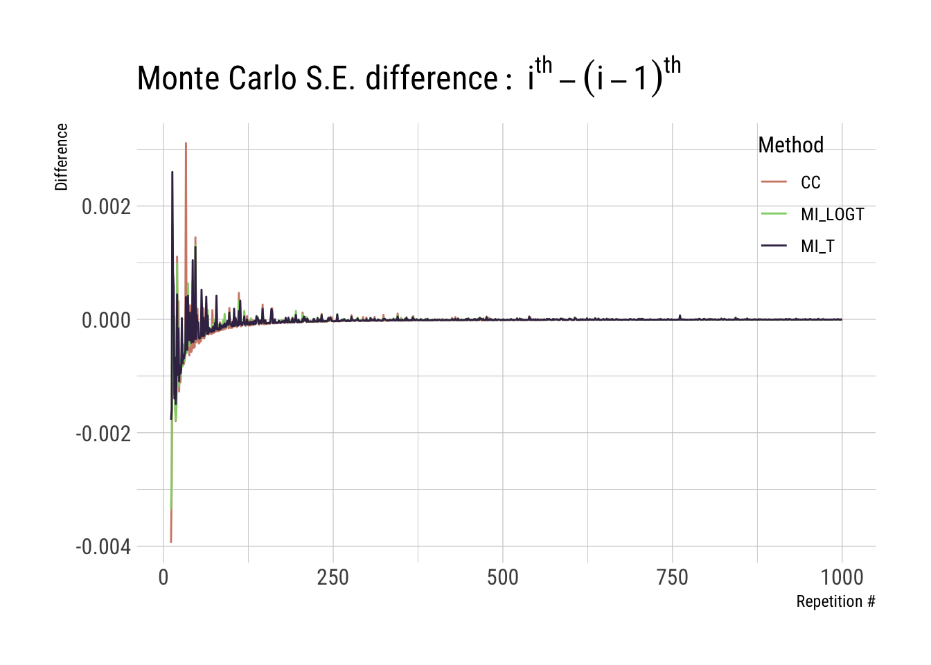
Let’s, therefore, calculate this difference (e.g. bias at i^th iteration versus bias at the (i-1)^th iteration), and let’s do it for both estimated bias and Monte Carlo standard error:

full_results <- arrange(full_results, method, i) %>%
  group_by(method) %>%
  mutate(
    lag_est = lag(est),
    lag_mcse = lag(mcse),
    diff_est = est - lag_est,
    diff_mcse = mcse - lag_mcse
  )

This difference is what we now decide to plot:

p1 <- ggplot(full_results, aes(x = i, y = diff_est, color = method)) +
  geom_line() +
  scale_color_ipsum() +
  theme_ipsum_rc(base_size = 12) +
  theme(legend.position = c(1, 1), legend.justification = c(1, 1)) +
  labs(x = "Repetition #", y = "Difference", color = "Method", title = expression(Bias ~ difference:~ i^th - (i - 1)^th))
p1

p2 <- ggplot(full_results, aes(x = i, y = diff_mcse, color = method)) +
  geom_line() +
  scale_color_ipsum() +
  theme_ipsum_rc(base_size = 12) +
  theme(legend.position = c(1, 1), legend.justification = c(1, 1)) +
  labs(x = "Repetition #", y = "Difference", color = "Method", title = expression(Monte ~ Carlo ~ S.E. ~ difference:~ i^th - (i - 1)^th))
p2

We save both plot objects p1 and p2, as we might be using that again later on. What we want here are the curves to flatten around zero, which seems to be the case for this example.

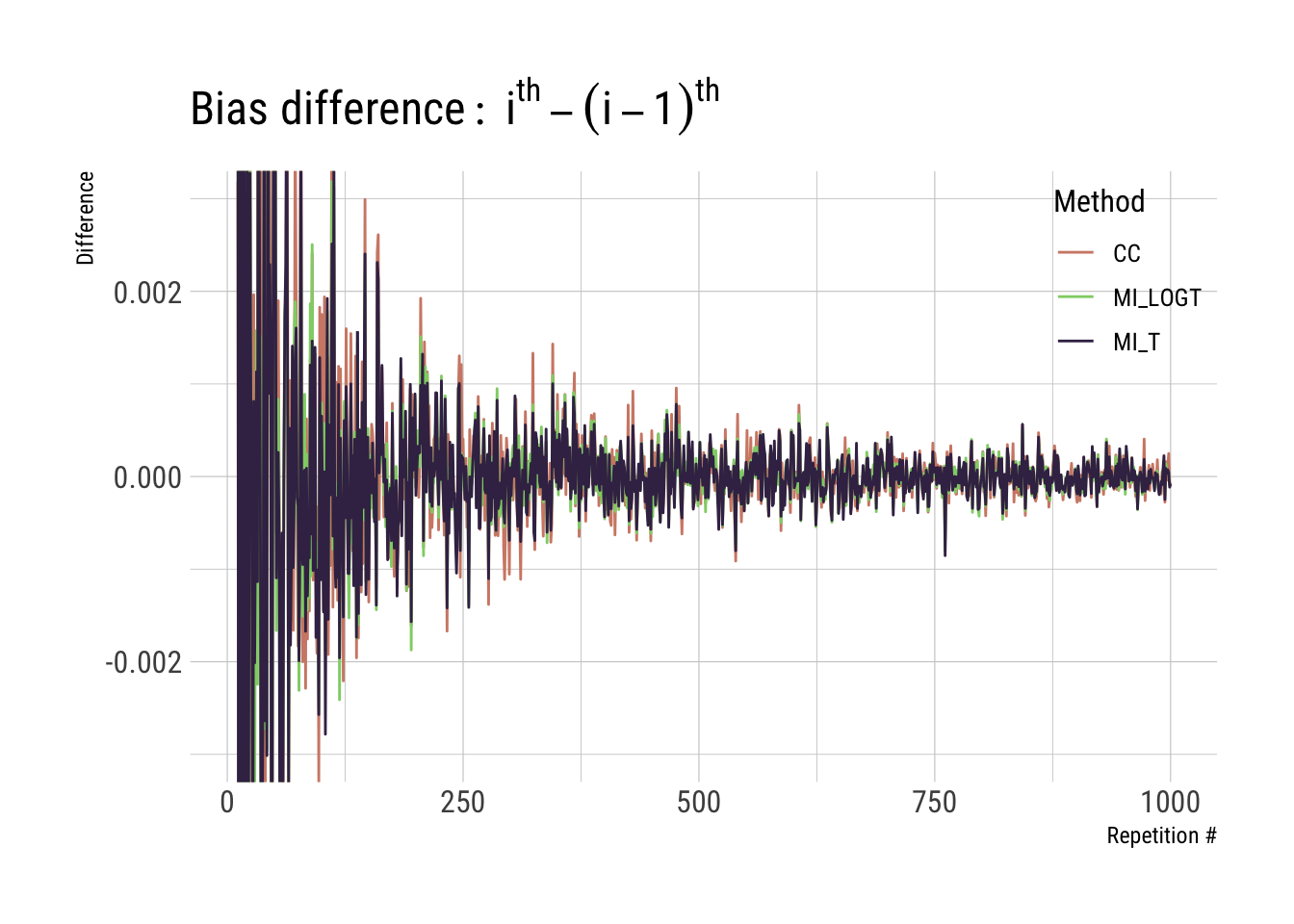
The y-scale of the plot is highly influenced by larger differences early on, so we could decide to focus on a narrower range around zero, e.g. for point estimates:

p1 + coord_cartesian(ylim = c(-0.003, 0.003))

With this, we can confirm what we suspected a few plots ago: that yes, the incremental value of running more than ~500 repetitions is somewhat marginal here.

To wrap up, there is one final thing I would like to mention here: all we did is post-hoc. We already run the study, hence all we get to do is to check whether the results are stable and precise enough (in our loose terms defined above).

The implication is an interesting one, in my opinion: you do not need a bunch of iterations if you can avoid it, especially if each repetition is expensive (computationally speaking).

What you could do, if you really wanted to, is to define a stopping rule such as:

After N (e.g. 10) consecutive iterations with a difference below a certain threshold (for the key performance measure), stop the study;
After you reach a given precision for bias (in terms of Monte Carlo error), stop the study;
You name it.

Of course, there are other things to consider such as the sequentiality of repetitions, especially if there are missing values (e.g. due to non-convergence of some iterations) – this is not meant to be, in any way, a comprehensive take on the topic. Feel free to reach out, as always, if you have any comments. Nevertheless, I think I will get back to this topic eventually, so stay tuned for that.

That’s all from me for today, then it must be closing time: talk to you soon and, in the meantime, take care!