Simulation and Twitter riddles

We use simulation and R to solve real-world problems.

Hi everyone!

Earlier today I stumbled upon this tweet by Sean J. Taylor:

Without doing the math or looking it up, approximately how many coin flips do you need to observe in order to be 95% confident you know Prob(Heads) to within +/- 1%?

— Sean J. Taylor (@seanjtaylor) April 22, 2021

…and I asked myself:

Can we answer this using simulation?

The answer is that yes, yes we can! Let’s see how we can do that using R (of course). Looks like this is now primarily a statistical simulation blog, but hey…

Let’s start by loading some packages and setting an RNG seed for reproducibility:

library(tidyverse)
library(hrbrthemes)
set.seed(3756)

Then, we define a function that we will use to replicate this experiment:

simfun <- function(i, .prob, .diff = 0.02, .N = 100000, .alpha = 0.05) {
  draw <- rbinom(n = .N, size = 1, prob = .prob)
  df <- tibble(
    n = seq(.N),
    x = cumsum(draw),
    mean = x / n,
    lower = (1 + (n - x + 1) / (x * qf(.alpha / 2, 2 * x, 2 * (n - x + 1))))^(-1),
    upper = (1 + (n - x) / ((x + 1) * qf(1 - .alpha / 2, 2 * (x + 1), 2 * (n - x))))^(-1),
    width = upper - lower
  )
  out <- tibble(i = i, prob = .prob, diff = .diff, y = min(which(df$width <= .diff)))
  return(out)
}

This function:

1. Repeates the experiment for 1 to 100,000 (.N) draws from a binomial distribution (e.g. our coin toss), with success probability .prob;

2. Estimates the cumulative proportion of heads (our ones) across all number of draws;

3. Estimates confidence intervals using the exact formula;

4. Calculates the width of the confidence interval. For a +/- 1% precision, that corresponds to a width of 2% (or 0.02, depending on the scale being used);

5. Finally, returns the first number of draws where the width is 0.02 (or less). This will tell us how many draws we needed to draw to get a confidence interval that is narrow enough for our purpose.

Then, we run the experiment B = 200 times, with different values of .prob (as we want to show the required sample sizes over different success probabilities):

B <- 200

results <- map_dfr(.x = seq(B), .f = function(j) {
  simfun(i = j, .prob = runif(1))
})

Let’s plot the results (using a LOESS smoother) versus the success probability:

ggplot(results, aes(x = prob, y = y)) +
  geom_point() +
  geom_smooth(method = "loess", size = 1, color = "#575FCF") +
  scale_x_continuous(labels = scales::percent) +
  scale_y_continuous(labels = scales::comma) +
  coord_cartesian(xlim = c(0, 1)) +
  theme_ipsum(base_size = 12, base_family = "Inconsolata") +
  theme(plot.margin = unit(rep(1, 4), "lines")) +
  labs(x = "Success probability", y = "Required sample size")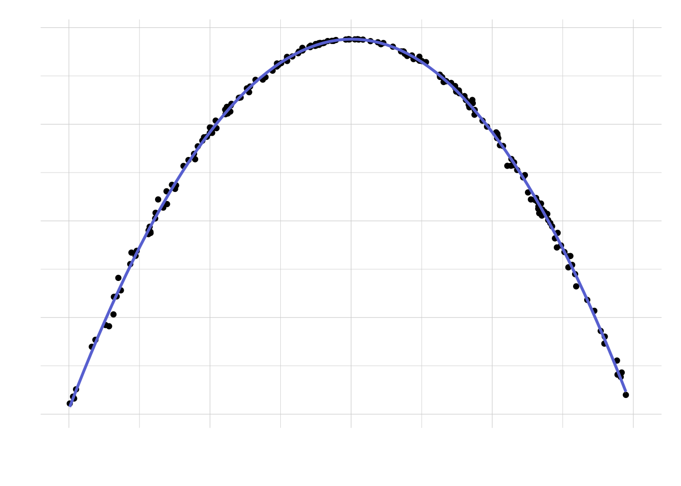

Looks like — as one would expect — the largest sample size required is for a success probability of 50%. What is the solution to the riddle then? As any statistician would confirm, it depends: if the coin is fair, then we would need approximately 10,000 tosses. Otherwise, the required sample size can be much smaller, even a tenth. Cool!

Finally, let’s repeat the experiment for a precision of +/- 3%:

results_3p <- map_dfr(.x = seq(B), .f = function(j) {
  simfun(i = j, .diff = 0.06, .prob = runif(1))
})

Comparing with the previous results (code to produce the plot omitted for simplicity):

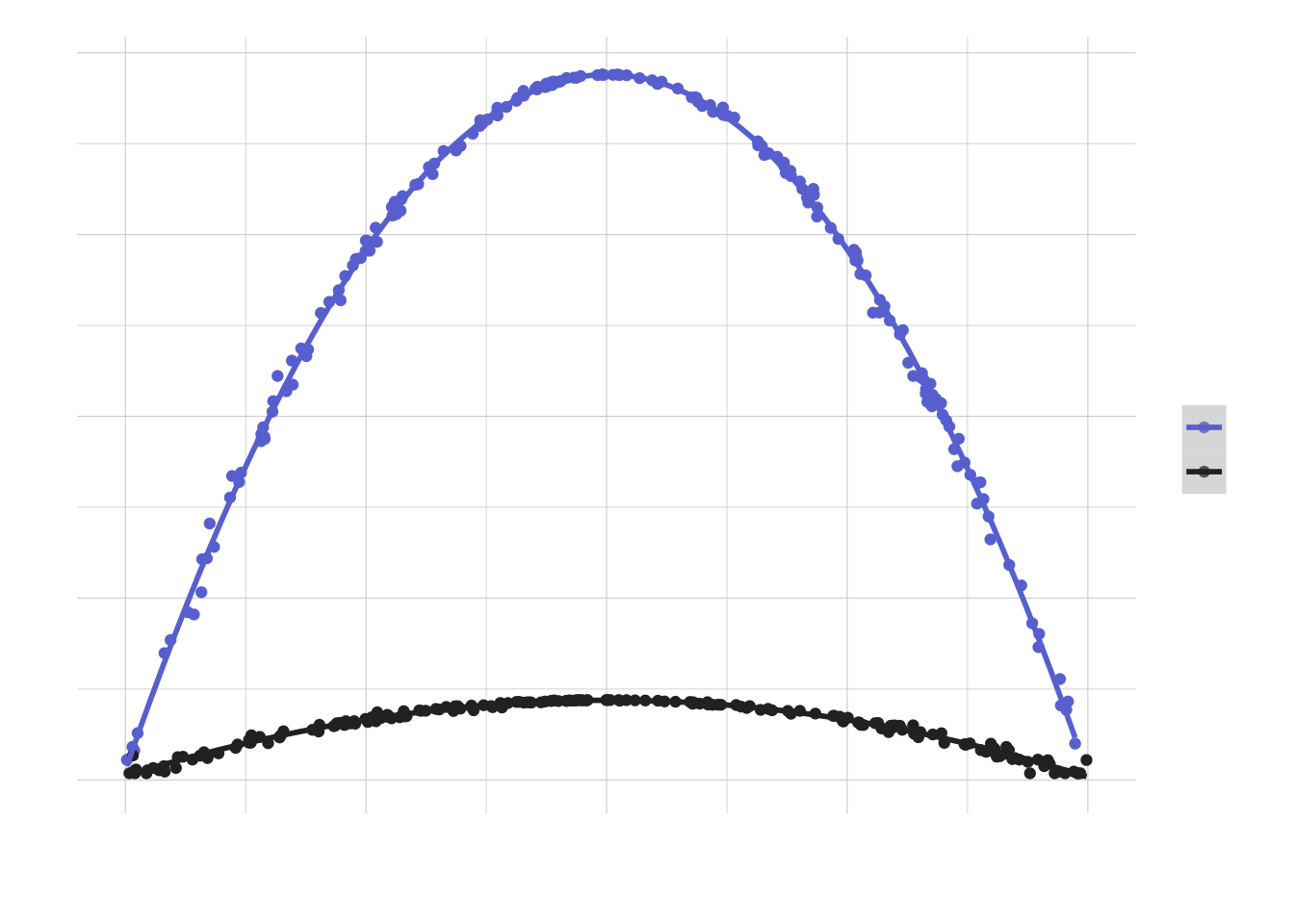
For a required precision of +/- 3% the sample size that we would need is much smaller, but the shape of the curve (i.e. versus the success probability) remains the same.

Finally, the elephant in the room: of course we could answer this using our old friend mathematics, or with a bit of Bayesian thinking. But where’s the fun in that? This simulation approach lets us play around with parameters and assumptions (e.g. what would happen if we assume a difference confidence level .alpha?), and it’s quite intuitive too. And yeah, let’s be honest: programming and running the experiment is just much more fun!

As always, please do point out all my errors on Twitter. Cheers!