Simulating survival times from a mixture cure model

This blog post illustrates how we could simulate survival times from a given mixture cure survival model using R.

Last Friday I was talking with a friend about simulating survival times from an experiment where most (if not all) events are happening within a short amount of time from inception. In other words, an experiment where the survival probability drops rapidly during the first days, staying then approximately flat until the end of the study.

This made me think about mixed cure fraction models, that is a model of the kind:

\[ S(t) = \pi + (1 - \pi) S_u(t) \]

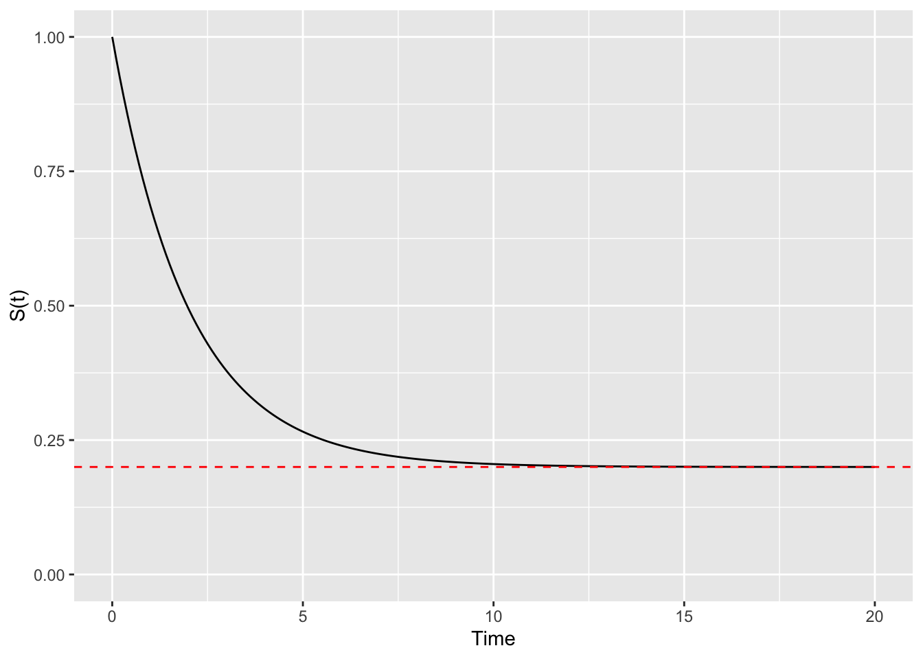
with \(\pi\) being the proportion cured and \(S_u(t)\) the survival function for the uncured subjects. Assuming \(S_u(t)\) follows an exponential distribution (for simplicity and from now onward), this corresponds to a survival curve like the following:

where \(\pi = 0.1\). With this model, the cure fraction creates an asymptote for the survival function, as \(100 \times \pi\)% of subjects are deemed to be cured; of course, \(\pi\) can be estimated from data. Interpretation of mixed cure fraction models is awkward, as one is assuming that subjects are split into cured and uncured at the beginning of the follow-up (which might not be the most realistic assumption), but discussing cure models is outside the scope of this blog post (and there are many papers you could find on the topic).

Back to the question, how to simulate from this survival function?

Well, as with most things these days, we can use the inversion method! First, we actually have to define which individuals are cured and which are not. To do so, we draw from a Bernoulli distribution with success probability \(\pi\):

set.seed(4875) # for reproducibility
n <- 100000
pi <- 0.2
cured <- rbinom(n = n, size = 1, prob = pi)
prop.table(table(cured))

cured
      0       1 
0.80074 0.19926 

Then, we simulate survival times e.g. from an exponential distribution (with \(\lambda = 0.5\)). We use the formulae described in Bender et al. (which is in fact the inversion method applied to survival functions):

lambda <- 0.5
u <- runif(n = n)
S <- -log(u) / lambda

Finally, we assign to cured individuals an infinite survival time (as they will not experience the event ever):

S[cured == 1] <- Inf

Of course, now we are required to censor individuals, say after 20 years of follow-up:

status <- S <= 20
S <- pmin(S, 20)
df <- data.frame(S, status)

…and there you have it, it’s done.

What we want to do next is checking that we are actually simulating from the model we think we are simulating from. Let’s first check by fitting a Kaplan-Meier curve:

library(survival)
KM <- survfit(Surv(S, status) ~ 1, data = df)
plot(KM)
abline(h = pi, col = "red")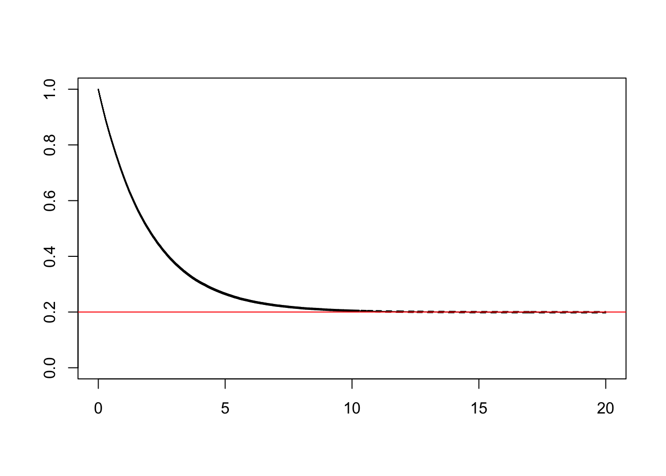

…which looks similar to the theoretical curve depicted above. Good!

Then, we could try to fit the data-generating model using maximum likelihood. The density function of the cure model is defined as

\[ f(t) = \frac{\partial F(t)}{\partial t} = (1 - \pi) \times f_u(t) \]

where \(F(t) = 1 - S(t)\) and \(f_u(t)\) is the density function for the non-cured subjects (e.g. from the exponential distribution, from our example above). Therefore, the likelihood contribution for the i^th subject can be defined as:

\[ L_i(\theta | t_i, d_i) = f(t_i)^{d_i} \times S(t_i)^{1 - d_i} \]

In R, that (actually, the log-likelihood) can be defined as:

log_likelihood <- function(par, t, d) {
  lambda <- exp(par[1])
  pi <- boot::inv.logit(par[2])
  f <- (1 - pi) * lambda * exp(-lambda * t)
  S <- pi + (1 - pi) * exp(-lambda * t)
  L <- (f^d) * (S^(1 - d))
  l <- log(L)
  return(-sum(l))
}

Some comments on the above function:

• I chose to model the parameter \(\lambda\) on the log-scale, and \(\pi\) on the logit scale. By doing so, we don’t have to constrain the optimisation routine to respect the boundaries of the parameters, as \(\lambda > 0\) and \(0 \le \pi \le 1\);

• f contains the density function of an exponential distribution (which is \(h(t) \times S(t)\));

• S contains the survival function of an exponential distribution;

• I take the log of the likelihood function (which generally behaves better when optimising numerically) and return the negative log-likelihood value (as R’s optim minimises the objective function by default).

Now, all we have to do is define some starting values stpar and then run optim.

stpar <- c(ln_lambda = 0, logit_pi = 0)
optim(par = stpar, fn = log_likelihood, t = df$S, d = df$status, method = "L-BFGS-B")

$par
 ln_lambda   logit_pi 
-0.6945243 -1.3909736 

$value
[1] 185584.3

$counts
function gradient 
       8        8 

$convergence
[1] 0

$message
[1] "CONVERGENCE: REL_REDUCTION_OF_F <= FACTR*EPSMCH"

The true values were:

log(lambda)

[1] -0.6931472

boot::logit(pi)

[1] -1.386294

…which (once again) are close enough to the fitted values. It does seem like we are actually simulating from the mixture cure model described above.

In conclusion, obviously this might not fit the actual experiment too well and therefore we might have to try other approaches before considering our work done. For instance, we could simulate from an hazard function that goes to zero after a given amount of time \(t^*\): this approach can easily be implemented using the {simsurv} package. The proof is left as an exercise for the interested reader.

Cheers!