library(haven)
brcancer <- read_dta("https://www.stata-press.com/data/r16/brcancer.dta")RMST and survival forests
rstats
survival-analysis
rmst
survival-forests
In this blog post we extend the approach that we used previously to calculate restricted mean survival time after fitting a random survival forest model.
This is a follow-up from my previous post on integrating survival curves and computing restricted mean survival times (RMST), which concluded with:
[…] it can be replicated with every model that yields predictions for the survival function \(S(t)\).
This made me think: can we actually compute the difference in RMST after fitting a random survival forest? Well, it turns out that yes, we can!
Let’s use the same dataset from the German breast cancer study:
We will be using the randomForestSRC package to fit a random survival forest. There are other options (such as the cforest function from the party package), but we’ll stick with randomForestSRC for simplicity.
library(randomForestSRC)The model we fit is the same model as before, with just treatment as a binary covariate:
set.seed(295682735)

fit <- rfsrc(Surv(rectime, censrec) ~ hormon, data = brcancer)
Again, for simplicity, we’ll use the default arguments of rfsrc (e.g. the number of trees to grow for the algorithm); we also set a seed for reproducibility. Let’s print the model fit:
fit Sample size: 686
Number of deaths: 299
Number of trees: 500
Forest terminal node size: 15
Average no. of terminal nodes: 2
No. of variables tried at each split: 1
Total no. of variables: 1
Resampling used to grow trees: swor
Resample size used to grow trees: 434
Analysis: RSF
Family: surv
Splitting rule: logrank *random*
Number of random split points: 10
(OOB) CRPS: 0.18779144
(OOB) Requested performance error: 0.64430821We don’t really care about the model accuracy here, as all of this is just a proof of concept.
randomForestSRC provides a predict method, which we can use to obtain prediction on a test dataset of two individuals (one treated, one untreated):
data_grid <- expand.grid(
  rectime = 1,
  censrec = 0,
  hormon = unique(brcancer$hormon)
)
fit_prediction <- predict(fit, newdata = data_grid)
We need to provide a value for rectime and censrec, despite it not being used by predict; by default, predictions are computed at each observed event time.
Interestingly, a variety of predictions are returned (e.g. survival probability, cumulative hazard, etc.). We can easily extract the survival predictions, which is a matrix with as many rows as individuals in the test dataset and as many columns as the number of distinct observed event times:
survival_prediction <- fit_prediction$survival

class(survival_prediction)
[1] "matrix" "array" dim(survival_prediction)[1] 2 150We process the prediction to be a tidy dataset:
# First reshape...
tidy_survival_prediction <- data.frame(fit_prediction$time.interest, t(survival_prediction))
names(tidy_survival_prediction) <- c("rectime", data_grid$hormon)
head(tidy_survival_prediction)
rectime 0 1
1 72 0.9976498 1.0000000
2 113 0.9930211 1.0000000
3 160 0.9883409 1.0000000
4 169 0.9883409 0.9959803
5 173 0.9834924 0.9959803
6 177 0.9811389 0.9875778# Second reshape...
library(tidyr)
tidy_survival_prediction <- pivot_longer(
tidy_survival_prediction,
cols = 2:3,
names_to = "hormon",
values_to = "S_hat_RF"
)
head(tidy_survival_prediction)# A tibble: 6 × 3
rectime hormon S_hat_RF
<dbl> <chr> <dbl>
1 72 0 0.998
2 72 1 1
3 113 0 0.993
4 113 1 1
5 160 0 0.988
6 160 1 1 # Adding a new factor for pretty plotting:
tidy_survival_prediction$hormon <- as.numeric(tidy_survival_prediction$hormon)
tidy_survival_prediction$hormon2 <- ifelse(tidy_survival_prediction$hormon == 0, "Control arm", "Treatment arm")We can finally plot the fitted survival curves from the random survival forest model:
library(ggplot2)
ggplot(tidy_survival_prediction, aes(x = rectime, y = S_hat_RF, linetype = hormon2)) +
  geom_line() +
  coord_cartesian(ylim = c(0, 1)) +
  scale_x_continuous(breaks = 365 * seq(6)) +
  theme(legend.position = c(0, 0), legend.justification = c(0, 0)) +
  labs(x = "Follow-up time (days)", y = "Fitted survival", linetype = "")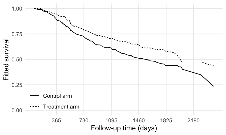
Not too bad!
Let’s now compute the fitted survival curves from the flexible parametric model, as a comparison:
# Fit...
library(rstpm2)
fit_rstpm2 <- stpm2(Surv(rectime, censrec) ~ hormon, data = brcancer, df = 5)

# Predict...
tidy_survival_prediction$S_hat_FPM <- predict(
  fit_rstpm2,
  type = "surv",
  newdata = tidy_survival_prediction
)

# ...and plot!
ggplot(tidy_survival_prediction, aes(x = rectime, linetype = hormon2)) +
  geom_line(aes(y = S_hat_RF, color = "Random forest")) +
  geom_line(aes(y = S_hat_FPM, color = "FPM")) +
  coord_cartesian(ylim = c(0, 1)) +
  scale_x_continuous(breaks = 365 * seq(6)) +
  scale_color_manual(values = c("red", "black")) +
  theme(legend.position = c(0, 0), legend.justification = c(0, 0)) +
  labs(x = "Follow-up time (days)", y = "Fitted survival", linetype = "", color = "")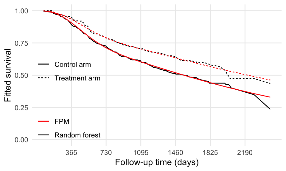
The two models seem to agree fairly well.
Let’s finally calculate the difference in RMST using the predictions from the random forest model:
idx_0 <- which(tidy_survival_prediction$hormon == 0 & tidy_survival_prediction$rectime <= 365 * 5)
df_0 <- tidy_survival_prediction[idx_0, ]
int_spline_0 <- splinefun(
  x = df_0$rectime,
  y = df_0$S_hat_RF,
  method = "natural"
)

idx_1 <- which(tidy_survival_prediction$hormon == 1 & tidy_survival_prediction$rectime <= 365 * 5)
df_1 <- tidy_survival_prediction[idx_1, ]
int_spline_1 <- splinefun(
  x = df_1$rectime,
  y = df_1$S_hat_RF,
  method = "natural"
)
Here we use the whole fitted survival curve to fit the spline interpolation. The RMST can finally be calculated as:
RMST_0 <- integrate(f = int_spline_0, lower = 0, upper = 365 * 5)$value
RMST_0
[1] 1262.283RMST_1 <- integrate(f = int_spline_1, lower = 0, upper = 365 * 5)$value
RMST_1[1] 1412.925The difference in RMST will therefore be RMST_1 - RMST_0 = 151 days, or equivalently, 0.413 years. Remember: using a flexible parametric model, the estimated difference in RMST was 140 days (0.382 years).
In conclusion, yes, it is possible to calculate RMST after fitting a random survival forest model. The example that was described above is kind of silly (I mean, we included a single binary covariate in a random forest model), but still kind of useful to illustrate how to do that in R. I guess I satisfied my curiosity — for now…