In this blog post, we will see how to use numerical integration to integrate survival curves in R.
Published
March 29, 2020
A survival curve \(S(t)\) represents the probability of a given event to happen at a given time point \(t\). It is often estimated using the Kaplan-Meier (product-limit) estimator.
However, sometimes it is useful to calculate the integral of a survival function, e.g. when computing restricted mean survival time.
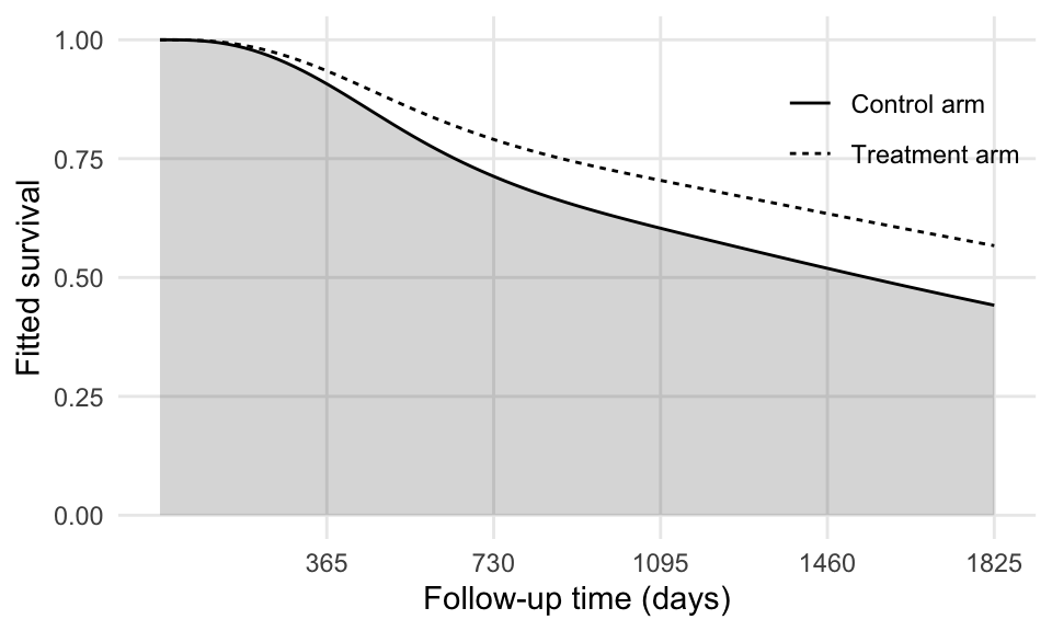
The restricted mean is a measure of average survival from time 0 to a specified time point, and may be estimated as the area under the survival curve up to that point.
Formally, the restricted mean survival time \(\mu\) is the mean of the survival time, limited to some horizon time \(t^*\). It equals the area under the survival curve \(S(t)\) from time zero to \(t^*\):
\[
\mu = \int_0^{t^*} S(u) \ du
\]
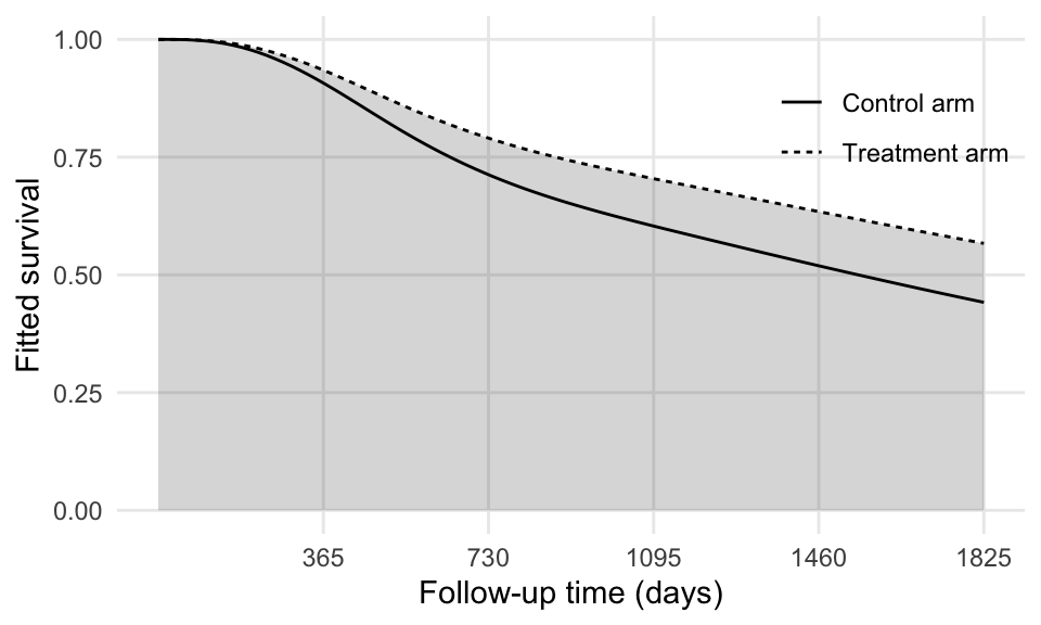
Most interestingly, the difference in restricted mean survival time between groups provides an alternative measure of treatment effect. Remember: the hazard ratio is not (in general) an appropriate measure of treatment effect in randomised trials with time to event outcomes.
The restricted mean survival time can be easily computed analytically if \(S(t)\) follows a (piecewise) exponential distribution. Otherwise, we can always compute the integral above numerically. The goal of this post is to show how to do so.
Data
Every example needs an example dataset: here I’ll be using data from the German breast cancer study, which comes bundled with Stata.
For simplicity, I will only include the treatment of interest (hormon, which represents hormonal therapy) as a covariate in the model. The survival time is rectime (in days), and the event indicator variable is censrec.
I am also creating a new variable hormon2 that will be useful for plotting:
The estimated hazard ratio is 0.695… but we don’t care about this measure, right?
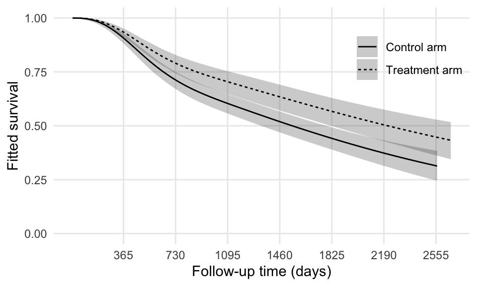
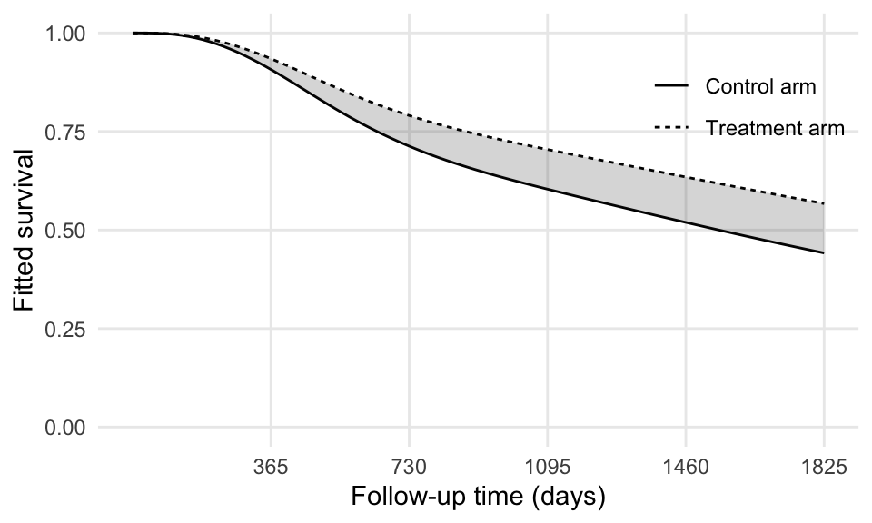
A benefit of modelling the baseline hazard (as compared to a Cox model) is that we can easily obtain smooth fitted survival curves for each combination of covariates of interest. For instance, the fitted survival curves for the two treatment arms are:
The fitted model is a flexible parametric model; in this setting, it is not straightforward to obtain an analytical solution.
We can, however, use spline-interpolation followed by numerical integration to compute the above integral very easily, and without needing to install any extra package. It will be a three-steps procedure:
We obtain a fine grid of predictions for each survival curve that we want to integrate (over follow-up time);
We obtain a function representing the spline interpolation of each curve;
We integrate the function that we just obtained.
Piece of cake!
Ok, there are four steps above, but don’t we deserve some cake?
Here we set \(t^*\) as 5 years, hence creating an appropriate grid for time and each treatment arm. Also, we start from .Machine$double.eps (roughly 2e-16) instead of zero as survival times need to be strictly positive; nevertheless, the difference will be negligible.
Then, onto step two. We predict the survival curve based on this grid:
data_grid$fitted <-predict(fit, newdata = data_grid, type ="surv")
Done.
Step three consists of fitting an interpolating spline for each fitted survival curve:
Here I am using a natural spline for the interpolation, but other methods work well too (in my experience) given that the function we are trying to interpolate is quite regular.
The cool thing about splinefun is that it returns a function that we can call. For instance, to obtain fitted (interpolated) survival at one year:
int_spline_0(365)
[1] 0.9072905
int_spline_1(365)
[1] 0.9346556
Finally, step four consist of using the built-in function integrate to (what a surprise!) integrate the two functions we just obtained:
We now have restricted mean survival time (in days) for both treatment arms:
RMST_0
[1] 1266.97
RMST_1
[1] 1406.486
In years, that will be:
RMST_0 /365
[1] 3.471151
RMST_1 /365
[1] 3.853386
Calculating the difference between the two is now trivial:
RMST_1 - RMST_0
[1] 139.5155
(RMST_1 - RMST_0) /365
[1] 0.3822341
Turns out, women treated with hormonal therapy have a 0.382-years longer time to recurrence compared to controls (and focussing on the first five years of follow-up only). Cool!
We would need to quantify the uncertainty in our estimate (and there is a closed-form formula for the standard error of the difference), but that’s a lesson for another day.
What are we actually calculating?
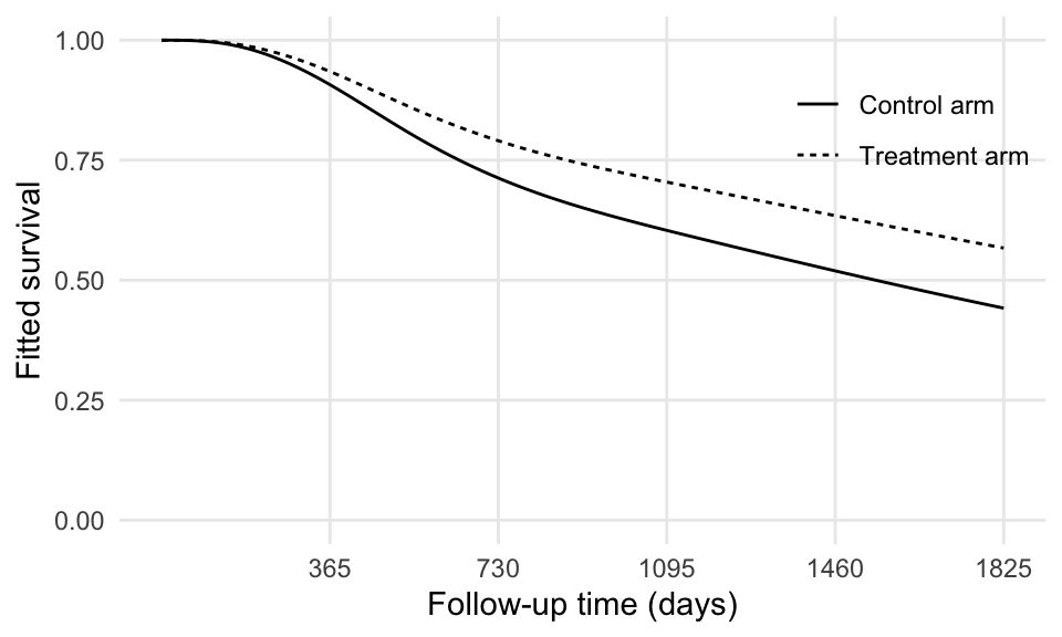
The two fitted survival curves that we are comparing are the following:
data_grid_diff is a dataset that was reshaped for plotting purposes, but otherwise contains the same information of data_grid.
Wrapping up
This post showed how to compute restricted mean survival time after fitting a flexible parametric model, but it can be replicated with every model that yields predictions for the survival function \(S(t)\).
I started writing this blog post with the idea of describing how to integrate survival functions in general terms but got carried away with the estimation of restricted mean survival time. Nevertheless, knowing how to integrate a survival function can be broadly useful e.g. when comparing different predictions from competing models or when comparing with the truth (if known, as in simulation studies). And it’s terribly easy!
This example used functions that come bundled with R for simplicity, but other functions and packages can be used as well. For instance, I prefer using the quadinf function from the pracma package for numerical integration, as I found it (empirically, of course) to be more robust and reliable than integrate. Other approaches for numerical integration can be used as well, such as Gaussian quadrature or more simple trapezoidal rules (and so on).
As always, let me know if I got something horribly wrong. Cheers!