rsimsum 0.8.0

Introducing the latest release of the {rsimsum} package, version 0.8.0.

I am glad to announce that a new release of rsimsum just landed on CRAN. And unlike leap years, this comes only 109 days after the last release! There is a lot of new stuff with this release, so buckle up.

The improvements coming with this release can be broadly categorised in two groups: enhanced flexibility, and new plots. Because who doesn’t like more plots?

Oh, and rsimsum comes with a new dataset too:

library(rsimsum)
data("tt", package = "rsimsum")

This is a toy simulation study to assess the robustness of the t-test to assumptions of equal variance and normality of the data. You can read more about it here.

Full Flexibility

We will use the t-test data to illustrate the new features.

The main function simsum now doesn’t require any more passing estimates standard errors (the se argument), nor a true value of the estimand (true argument):

s1 <- simsum(data = tt, estvarname = "diff")
summary(s1)

Values are:
    Point Estimate (Monte Carlo Standard Error)

Non-missing point estimates/standard errors:
 Estimate
     4000

Average point estimate:
 Estimate
  -0.9988

Median point estimate:
 Estimate
  -0.9551

Empirical standard error:
        Estimate
 1.6208 (0.0181)

As you can see, now simsum will do what it can with the information provided and compute only summary statistics that do not require standard errors nor the true value.

We can of course pass only one of se and true:

s2 <- simsum(data = tt, estvarname = "diff", se = "se")
summary(s2)

Values are:
    Point Estimate (Monte Carlo Standard Error)

Non-missing point estimates/standard errors:
 Estimate
     4000

Average point estimate:
 Estimate
  -0.9988

Median point estimate:
 Estimate
  -0.9551

Average variance:
 Estimate
   2.1956

Median variance:
 Estimate
   1.7171

Empirical standard error:
        Estimate
 1.6208 (0.0181)

Model-based standard error:
        Estimate
 1.4818 (0.0070)

Relative % error in standard error:
         Estimate
 -8.5785 (1.1107)

Bias-eliminated coverage of nominal 95% confidence interval:
        Estimate
 0.9233 (0.0042)

Power of 5% level test:
        Estimate
 0.1370 (0.0054)

s3 <- simsum(data = tt, estvarname = "diff", true = -1)
summary(s3)

Values are:
    Point Estimate (Monte Carlo Standard Error)

Non-missing point estimates/standard errors:
 Estimate
     4000

Average point estimate:
 Estimate
  -0.9988

Median point estimate:
 Estimate
  -0.9551

Bias in point estimate:
        Estimate
 0.0012 (0.0256)

Relative bias in point estimate:
         Estimate
 -0.0012 (0.0256)

Empirical standard error:
        Estimate
 1.6208 (0.0181)

Mean squared error:
        Estimate
 2.6264 (0.0684)

Each call to simsum will compute only the summary statistics that can actually be calculated with that provided!

Then, why stop with passing a single value of true only? What if your simulation study had a different true value of your estimand per each replication? Well, simsum now has you covered, pal.

The true argument of simsum can now be a string that identifies a column in data:

tt$true <- -1
s4 <- simsum(data = tt, estvarname = "diff", true = "true")
summary(s4)

Values are:
    Point Estimate (Monte Carlo Standard Error)

Non-missing point estimates/standard errors:
 Estimate
     4000

Average point estimate:
 Estimate
  -0.9988

Median point estimate:
 Estimate
  -0.9551

Bias in point estimate:
        Estimate
 0.0012 (0.0256)

Relative bias in point estimate:
         Estimate
 -0.0012 (0.0256)

Empirical standard error:
        Estimate
 1.6208 (0.0181)

Mean squared error:
        Estimate
 2.6264 (0.0684)

all.equal(target = get_data(s3), current = get_data(s4))

[1] TRUE

Beautiful!

Now that this was done, why stop here? Coverage probability is (by default) computed using the provided point estimates and standard errors, and computing symmetric confidence intervals that assume normality. What if you wanted to use asymmetric, replication-specific confidence limits instead? You guessed it: simsum got you covered too.

tt has two columns with each replication-specific confidence bounds of diff, lower and upper (who would have guessed, right?). You can pass these column names to simsum:

s5 <- simsum(data = tt, estvarname = "diff", se = "se", true = -1, ci.limits = c("lower", "upper"))
summary(s5, stats = "cover")

Values are:
    Point Estimate (Monte Carlo Standard Error)

Coverage of nominal 95% confidence interval:
        Estimate
 0.9290 (0.0041)

Compare with using the default settings:

s6 <- simsum(data = tt, estvarname = "diff", se = "se", true = -1)
summary(s6, stats = "cover")

Values are:
    Point Estimate (Monte Carlo Standard Error)

Coverage of nominal 95% confidence interval:
        Estimate
 0.9233 (0.0042)

In this case, it doesn’t really make a difference, but it is nice to have the option to do so if your simulation study requires it.

Of course, this all applies to multisimsum too (if you have several estimands at once). Check the new vignette on the topic for more details.

New Plots

rsimsum already supports a large variety of plots to quickly visualise the results of your simulation study. This release brings two new options: contour plots and hexbin plots.

These visualisations are useful to plot point estimates and standard errors when there is large overlap, as in the following example:

library(ggplot2)
data("MIsim", package = "rsimsum")
s <- simsum(data = MIsim, estvarname = "b", se = "se", true = 0.5, methodvar = "method", x = TRUE)
autoplot(s, type = "est")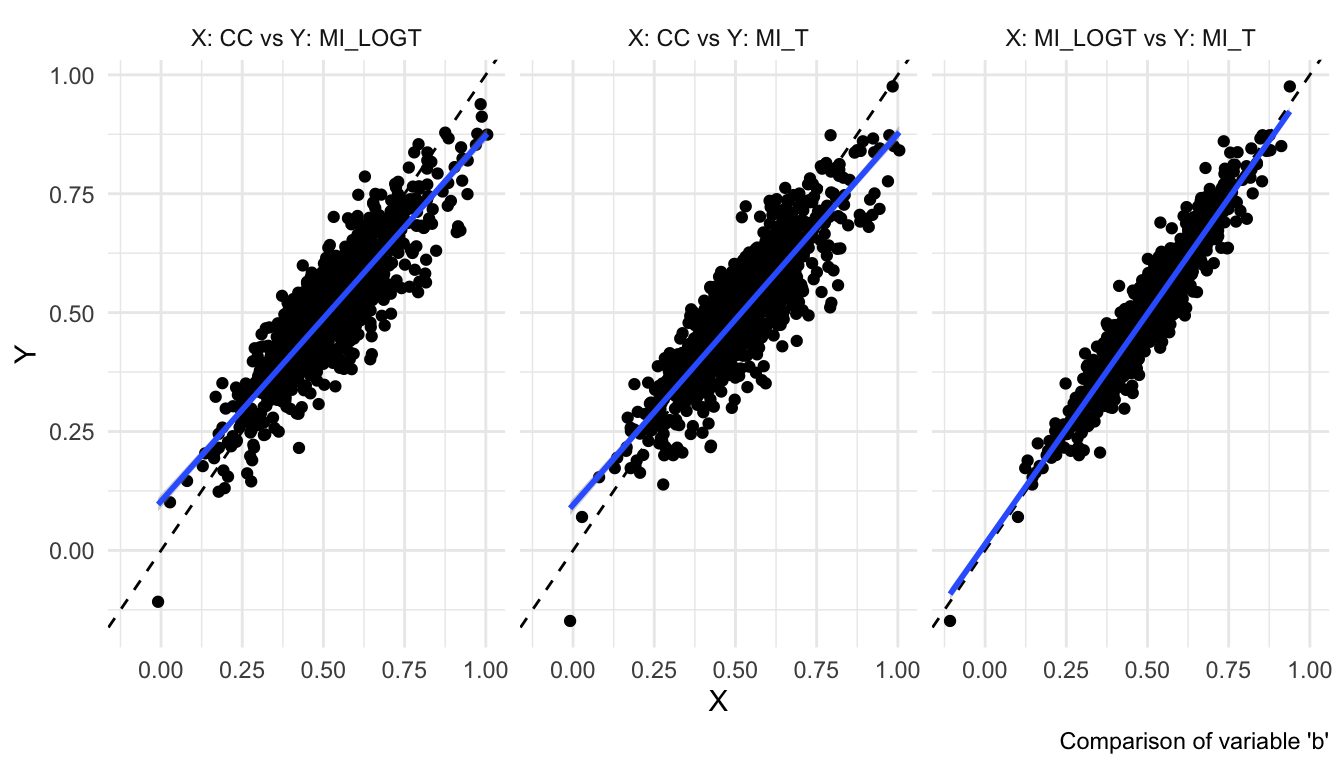

These plots are using theme_minimal() here, but will use the standard ggplot2 theme by default.

The same plot using contour lines is much more informative:

autoplot(s, type = "est_density")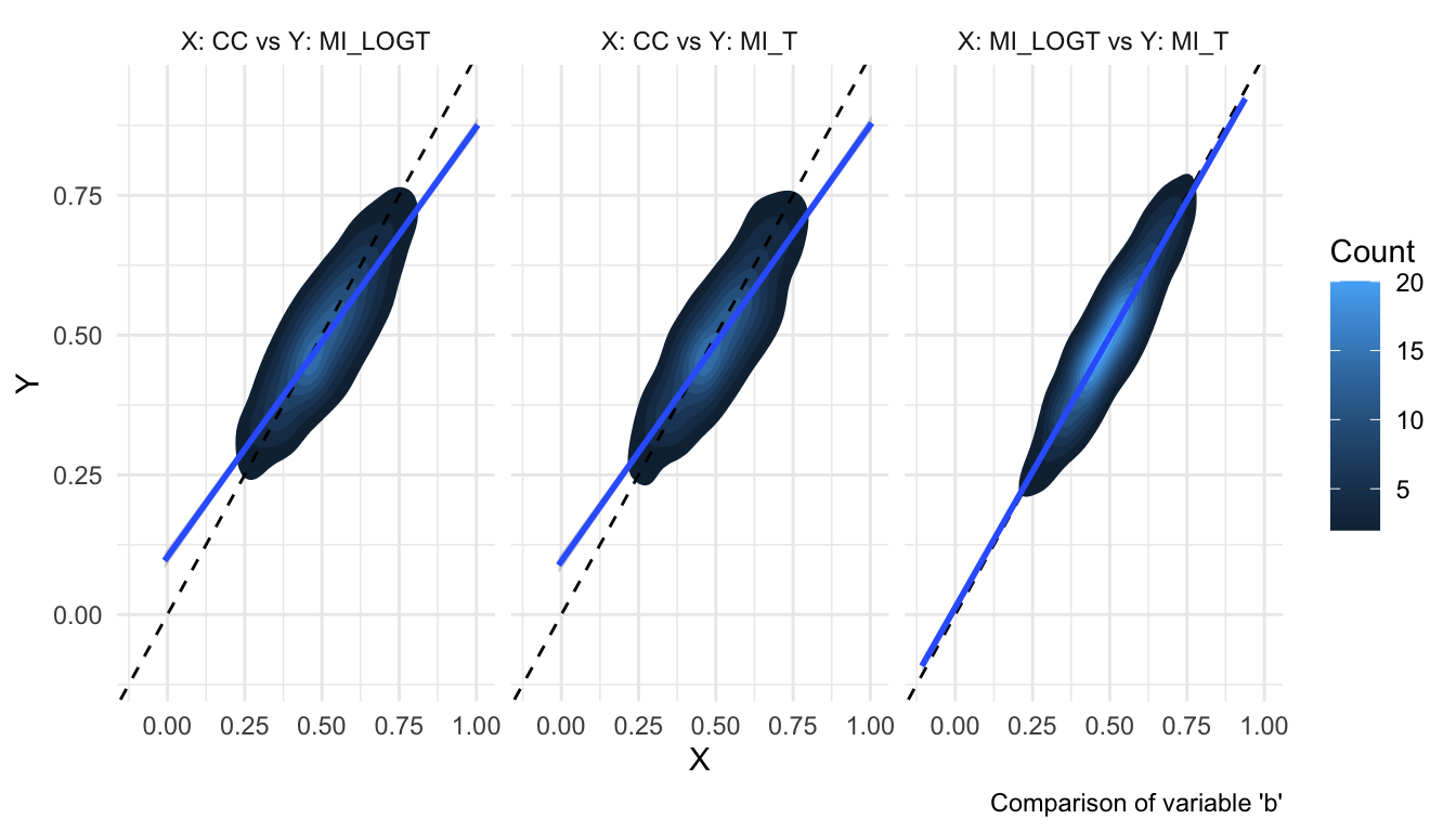

And given that everybody loves hexagons (looking at you, Tim), hexbin plots are now supported too:

autoplot(s, type = "est_hex")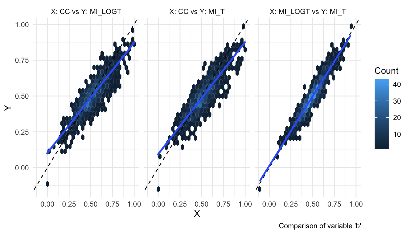

Finally, there is a new (and hopefully useful) feature for zip plots. By default, the whole range is plotted:

autoplot(s, type = "zip")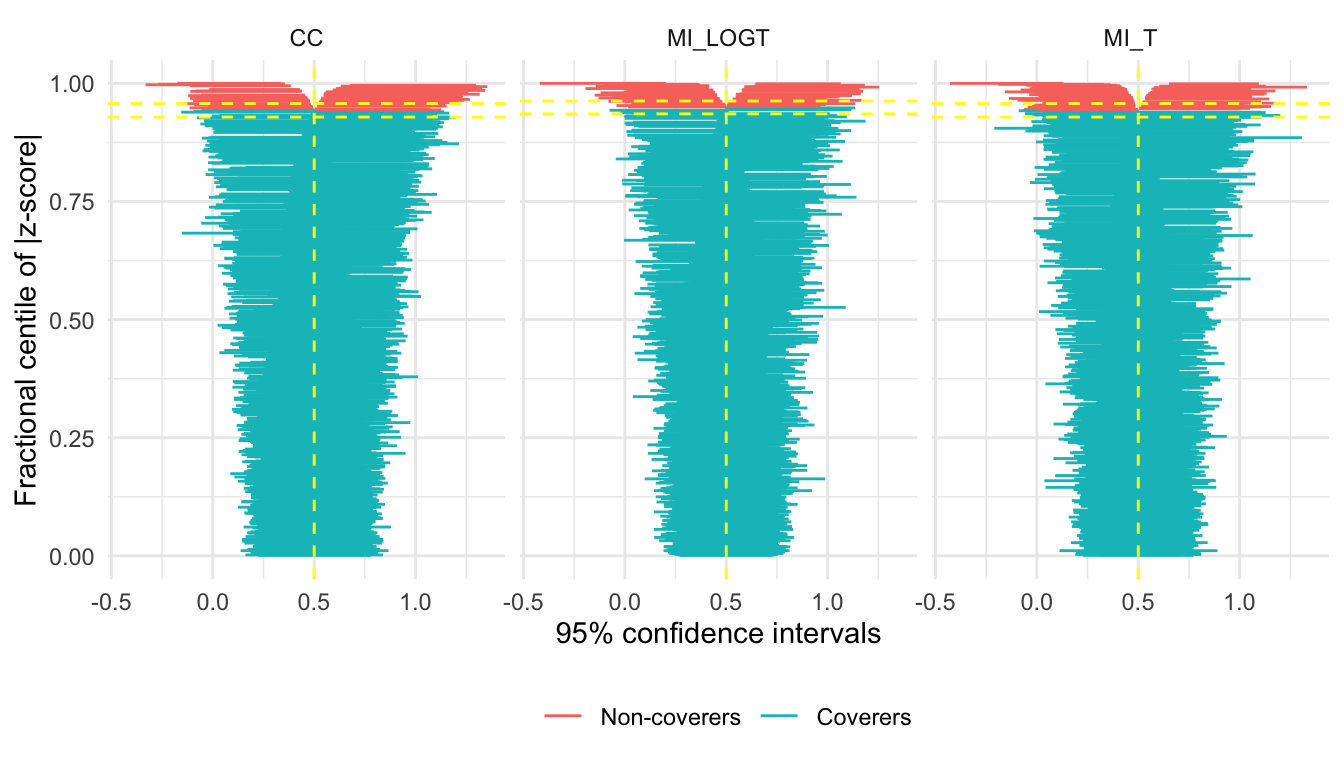

However, the bottom 90-ish percent of the plot is generally not very interesting. autoplot now accepts a zoom argument that allows zooming on the top x% of the zip plot:

autoplot(s, type = "zip", zoom = 0.1)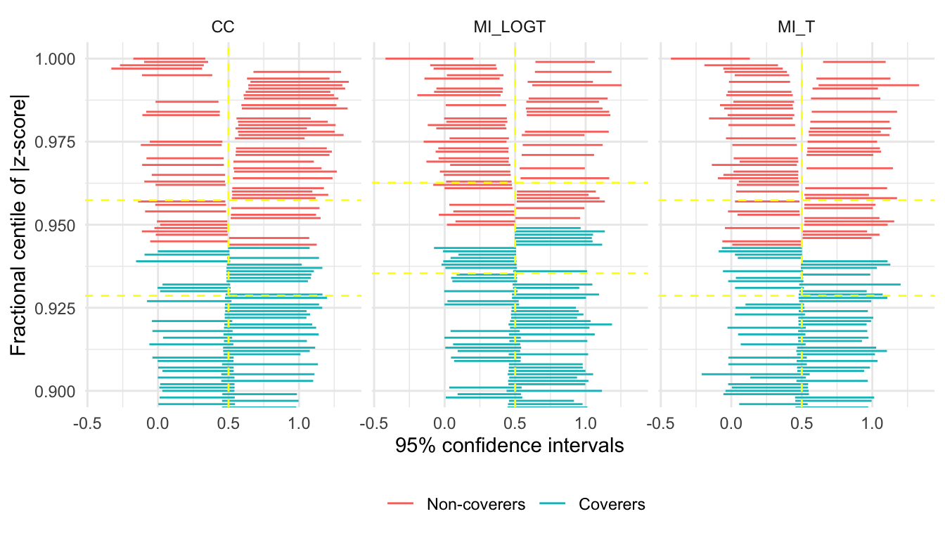

See that now we zoomed on the top 10% of the plot, making it much easier to notice differences between the methods.

Wrapping Up

This is all for now. As always, you can install the updated version from CRAN by typing the following in your R console:

install.packages("rsimsum")

Running update.packages() should work fine too.

Let me know if you spot any bugs by opening an issue on GitHub or e-mailing me directly.